Chapter 16 Boundary Element Method

Chapter 16 Boundary Element Method We will proceed to learn about Object Oriented Programming and Design by looking at a specific example that revolves around the solution of the Laplace equation by the Boundary Element Method (BEM). The benefits of this approach is that it takes a 2D or 3D PDE and reduces it to an algorithm that involves 1D or 2D computations only, respectively. For simplicity we will focus on the 2D case only.

16.1

The equations and the boundary conditions

The Laplace equation takes the form ∇2 φ = ∇ · (∇φ) = 0

(16.1)

subject to boundary conditions of the type 1. Dirichlet where the unknown function is imposed on a portion of the boundary, i.e. φ(x) = a(s), s being a coordinate system along the boundary. 2. Neumann where the normal derivative of the function is known ∇φ·n = q(s) where n is the outward unit normal. 3. Robin where a relationship of the form αφ + β∇φ · n = r(s). A well-posed problem requires the specification of only one type of boundary conditions on any portion of the boundary, that is either the function value is specified, or the normal derivative but not both. The data imposed on the boundary form are part of the problem’s specification and can be quite arbitrary except for some minor constraints. For example, if Neumann conditions are applied over the entire boundary, then the solution can be determined only up to an additive constant, that is if φ is a solution of ∇2 φ = 0 with ∇φ · n = q, then so is φ + C where C is an 155

156

CHAPTER 16. BOUNDARY ELEMENT METHOD arbitrary constant. In that case the flux have to satisfy a compatability condition that can be derived by applying the divergence theorem to equation 16.1: Z Z Z ∇2 φ dA = ∇φ · n ds = q ds = 0 (16.2) ∂Ω

Ω

16.2

∂Ω

From PDE to Integral Equation

Consider a function G, solution to a Poisson equation of the form: ∇2 G = Q(x − xi )

(16.3)

where Q(x − xi ) is a function that depends on the space variable x and on the source point xi where an impulse forcing is applied. I will keep these terms vague for the time being, and will delay specifying them until later. Multiplying equation 16.3 by φ and 16.1 by G and substracting the resulting expressions we get: φ∇2 G − G∇2 φ = φG(x − xi )

(16.4)

Integrating the above equation over the area of the domain Ω we get: Z

2

Ω

2

(φ∇ G − G∇ φ) dA =

Z

Ω

φG(x − xi ) dA

(16.5)

The chain rule of differentiation and the Gauss divergence theorem can be used to turn the left hand side into a boundary integral only. Indeed since for any differentiable functions a and b: ∇ · (a∇b) = ∇a · ∇b + a∇2 b, we can then write: φ∇2 G − G∇2 φ = ∇ · (φ∇G) − ∇φ · ∇G − ∇ · (G∇φ) + ∇φ · ∇G (16.6) = ∇ · (φ∇G) − ∇ · (G∇φ) = ∇ · (φ∇G − G∇φ) (16.7) Furthermore the divergence form of the last equations permits the application of the Gauss divergence theorm to get:

Z

Z

(φ∇2 G − G∇2 φ) dA = Ω

∇ · (φ∇G − G∇φ) dA =

ZΩ

∂Ω

Z

n · (φ∇G − G∇φ) dS =

∂Ω

∂φ ∂G −G φ ∂n ∂n

!

dS =

Z

ZΩ

ZΩ

Ω

Z

Ω

φQ(x − xi ) dA

(16.8)

φQ(x − xi ) dA

(16.9)

φQ(x − xi ) dA

(16.10)

φQ(x − xi ) dA

(16.11)

Further progress can be made to simplify equation 16.11 by imposing constraints on the choices of Q and G. Requiring that the function Q be the equivalent of the two-dimensional Dirac delta function, and G to be its associated free space

157

16.3. THE FREE SPACE GREEN FUNCTION

Green function allows us to reduce the integral on the right hand side of 16.11, since by definition: Z φQ(x − xi ) dA = φ(xi ) (16.12) Ω

Equation 16.11 becomes

∂φ ∂G −G φ ∂n ∂n

Z

∂Ω

!

dS = φ(xi )

(16.13)

Equation 16.13 is the starting point of the boundary element method. It essentially implies that if the unknown function φ and its normal derivative are known at the boundaries, then the solution at any point in the interior can be calculated. The rub is that for any well-posed problem the function φ or its normal derivative is known at the boundary but not both. The next step is then to use the above formulation to determine the missing data on the boundary; once the boundary data is known fully the solution in the interior can be calculated simply by moving the source point xi to any point where the solution is desired. The strategy for determining the missing data on the boundary starts by moving the source point to the boundary, and setting the equation purely in terms of the boundary unknowns. The equation is then term an integral equation. Prior to presenting the discretization of this integral equation, we take a detour to determine the Green function and its properties.

16.3

The Free Space Green Function

The free space Green function is by definition the solution to a forced problem with homogeneous forcing, except for a single impulse of infinite magnitude in an unbounded domain. The derivation proceeds by setting the Laplace equation in polar coordinates: 1 ∂2φ ∂ 2 φ 1 ∂G + 2 2 (16.14) ∇2 G = 2 + ∂r r ∂r r ∂θ The function G is defined on an unbounded domain with zero forcing except at a single point, we thus expect G to depend only on the distance to the point xi 2 but not on the angle θ, so that ∂∂θφ2 = 0. The two-dimensional form of the Dirac delta function can be built from its one-dimensional counterpart: δ(x); the latter is defined as δ(x) =

(

0 x 6= 0 ∞ x=0

with

Z

∞

δ(x) dx = 1.

(16.15)

−∞

In particular we have for any function f (x) that Z

∞

f (x)δ(x − x0 )dx = f (x0 ) −∞

(16.16)

158

CHAPTER 16. BOUNDARY ELEMENT METHOD

One may wonder how to define a function which vanishes everywhere, spikes to infinity at a single point, and yet has unit area under the curve. A simple example is given by the function δa = max(0, (a − |x|)/a2 ), and taking its limit as a → 0. In 2D the definition of the function differs a bit from its one-dimensional counterpart. In particular setting δ(r) Q(x, xi ) = , (16.17) 2πr where r = |x − xi | is the distance of the point x from the source point xi . It is easy to verify that the area under Q is unity, indeed we have Z

A

Q(x)dA =

Z

2π

0

Z

0

∞

δ(r) r dr dθ = 1 2πr

(16.18)

We are now ready to determine our free space Green function. Dropping the azimuthal dependency from the Laplacian in polar coordinates we have ∂ 2 φ 1 ∂G + ∂r 2 r ∂r! 1∂ ∂G r rr ∂r ∂G r ∂r ∂G r ∂r ∂G ∂r

= = = = =

G =

δ(r) 2πr δ(r) 2πr Z δ(r) dr 2π 1 +A 2π 1 A + 2πr r ln |r| + A ln |r| + B 2π

(16.19) (16.20) (16.21) (16.22) (16.23) (16.24)

where A and B are integration constants. The constant B is just an offset to the function, and we can arbitrarily set it to 0. The constant A can be determined by an application of the divergence theorem on a circle of radius R we then have Z

A

Q dA =

Z

A

∇2 GdA =

Z

∂A

Z 2π ∂G ∂G ds = Rdθ = 1 + 2πA ∂n ∂r 0

(16.25)

Since the left hand side of the equation is equal to 1, the constant A = 0. A final note concerns the case where the source point is located on the boundary of the domain. The integral takes then a slightly different form. Figure 16.1 shows a sketch with the source point on the boundary. The area integral is now divided into a piece that excludes the point plus an infinitesimally small area near the source. The first integral is of couse zero while the second leads to Z

0

α

Z

ǫ 0

φ(x)

α δ(r) r dr dθ = φ(xi ) 2πr 2π

(16.26)

159

16.4. DISCRETIZATION

s

n

j+1

j r

i

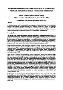
Figure 16.1: BEM discretization of the geometry with straight line segments. The source point is located at xi while the field points cover segement sj ≤ s ≤ sj+1 . where α is the interior angle of the boundary. If the boundary is a smooth curve α = π. Our final form for equation 16.27 becomes Z

∂Ω

∂G ∂φ φ −G ∂n ∂n

!

dS =

α φ(xi ), 2π

G=

ln |r| 2π

(16.27)

or equivalently !

∂φ φ ∂r dS = αφ(xi) (16.28) − ln |r| r ∂n ∂n ∂Ω where r is understood to be the disctance from the field point x to the source point xi . Z

16.4

Discretization

The discretization of the continuous problem proceeds by first dividing the boundary of the domain into line segments so that the geometry of the domain is wellrepresented. The choice of line type is rather arbitrary. In the following we will only consider the case where the line segments are straight lines as sketched in figure 16.1. Notice that for linear segments: r 2 = s2 + n2 , and

∂r n = ∂n r

(16.29)

160

CHAPTER 16. BOUNDARY ELEMENT METHOD

The boundary integral can now be changed to a discretization over the individual segments so that equation 16.28 becomes N Z X

sj+1

j=1 sj

1 ∂φ n − ln(s2 + n2 ) φ 2 2 n +s 2 ∂n

!

ds = αφ(xi )

(16.30)

The second piece of the discretization is to approximate the variations of φ and its normal derivative ∇φ · n on the boundary. Again, different choices lead to different formulations, here we will use a basic linear variations between the nodes so that s − sj sj+1 − s φj+1 + φj ∆s ∆s sj+1 − s ∂φ ∂φ s − sj ∂φ + (s) = ∂n ∆s ∂n j+1 ∆s ∂n j φ(s) =

(16.31) (16.32)

with ∆s = sj+1 − sj being the length of the boundary segment j. Note that the φj and ∂φ are just coefficients that will be chosen to enforce the integral equations. ∂n j Replacing the approximations in equation 16.30 we get N X

Z

sj

j=1 N X

j=1

 

sj+1

Z

sj+1

sj

sj+1 − s s − sj n φj+1 + φj 2 2 n +s ∆s ∆s 





!

ds − αφ(xi ) = 



1 sj+1 − s ∂φ  s − sj ∂φ + ds = ln(s2 + n2 )  2 ∆s ∂n j+1 ∆s ∂n j

(16.33)

The above equation is nothing but a row of the matrix equation governing the relationship between φ and its normal derivative. A more compact form is: N X

(Ki,j φj + Ki,j+1φj+1 ) − αφ(xi ) =

N X

j=1

j=1

with

Ri,j Ri,j+1

Ri,j



Z





∂φ ∂φ  + Ri,j+1 ∂n j ∂n j+1

n sj+1 sj+1 − s ds ∆s sj n2 + s2 Z n sj+1 s − sj = ds ∆s sj n2 + s2 Z sj+1 1 = (sj+1 − s) ln(s2 + n2 ) ds 2∆s sj 1 Z sj+1 = (s − sj ) ln(s2 + n2 ) ds 2∆s sj

Ki,j = Ki,j+1



(16.34)

(16.35) (16.36) (16.37) (16.38)

Notice that we have been able to pull n out of the integral because it is constant for the straight line approximation of the boundary curves.

161

16.4. DISCRETIZATION

16.4.1

Evaluation of Integrals

All the integrals in 16.35-16.38 can be evaluated analytically; indeed it is easy to verify that:  sj+1 s n Z sj+1 n 2 2 A(sj+1 , sj , n) = ds = ln(s + n ) ∆s sj n2 + s2 2∆s sj 2 rj+1 n ln 2 (16.39) = 2∆s rj  sj+1 Z 1 1 n sj+1 −1 s tan ds = B(sj+1 , sj , n) = ∆s sj n2 + s2 ∆s n sj   sj+1 sj 1 tan−1 (16.40) − tan−1 = ∆s n n 1 n∆s = (16.41) tan−1 ∆s 1 + sj sj+1 Z sj+1 1 s ln(s2 + n2 ) ds C(sj+1 , sj , n) = 2∆s sj isj+1 1 h 2 = (s + n2 ) ln(n2 + s2 ) − (s2 + n2 ) sj 4∆s   i 1 h 2 2 2 = rj+1 ln rj+1 − rj+1 − rj2 ln rj2 − rj2 (16.42) 4∆s Z sj+1 1 ln(s2 + n2 ) ds D(sj+1 , sj , n) = 2∆s sj  sj+1 1 2 2 −1 s = s ln(n + s ) − 2s + 2n tan 2∆s n sj   1 2 −1 sj+1 sj+1 ln rj+1 − 2sj+1 + 2n tan = 2∆s n   2 −1 sj (16.43) − sj ln rj − 2sj + 2n tan n   1 sj+1 2 = sj+1 ln rj+1 + 2n tan−1 2∆s n   s j −1 (16.44) − sj ln rj2 + 2n tan−1 n " # 1 n∆s 2 = sj+1 ln rj+1 − sj ln rj2 + 2n tan−1 −1 2∆s 1 + sj sj+1 tan x−tan y where we have used the fact that tan(x−y) = 1+tan to simplify the expressions. x tan y Replacing these expressions into the definition of the matrix entries we have

Ki,j = Ki,j+1 = Ri,j = Ri,j+1 =

sj+1 B(sj+1, sj , n) − A(sj+1 , sj , n) −sj B(sj+1 , sj , n) + A(sj+1, sj , n) sj+1 D(sj+1, sj , n) − C(sj+1, sj , n) −sj D(sj+1, sj , n) + C(sj+1 , sj , n)

(16.45) (16.46) (16.47) (16.48)

162

CHAPTER 16. BOUNDARY ELEMENT METHOD

Notice that special care must be taken when integrating along an edge that contains the source point, since in that case either rj or rj+1 is zero. To account for this case we notice first that when n = 0 we have A(sj+1, sj , 0) = 0 B(sj+1, sj , 0) = 0

(16.49) (16.50)

  i 1 h 2 sj+1 ln s2j+1 − s2j+1 − s2j ln s2j − s2j (16.51) 4∆s i 1 h D(sj+1, sj , 0) = sj+1 ln s2j+1 − sj ln s2j − 1 (16.52) 2∆s In a second step it is now easy to take the limit when sj or sj+1 are zero, since x ln x → 0 when x → 0, and so we have: sj (2 ln sj − 1) (16.53) C(0, sj , 0, 0) = 4 sj+1(2 ln sj+1 − 1) C(sj+1 , 0, 0) = (16.54) 4 D(0, sj , 0) = ln sj − 1 (16.55) D(sj+1 , 0, 0) = ln sj+1 − 1 (16.56)

C(sj+1, sj , 0) =

16.5

Algorithm

The development of a code for solving the Laplace equation on arbitrary domain using BEM requires several steps: 1. Description of the geometry 2. Description of the boundary conditions 3. Building the matrices mostly by evaluating integrals 4. Constructing of the linear system by assembly 5. Solution of the linear system 6. Evaluating the solution at interior points 7. Plotting the solution and displaying it. We will take up each of these tasks in the following subsections.

16.5.1

Geometry description

The geometry is essentially formed by a collection of nodes connected by edges. We can already envision a derived type called bemnode and a derived type called polygon made-up of a collection of bemnodes. The location of the nodes of each polygon must be read from files that contain the list of nodes and their attributes.

16.5. ALGORITHM

163

bemnode data type and functionality The bemnode data type must provide the following information: 1. The coordinates of the node list in an array of dimension \sdim; here sdim is parameter equal to 2 for 2D problems. 2. The type of boundary condition applied at the node. We will code that with an integer data type called bctype. 3. The value of the function and its normal derivative at the node. If these are not known, they should be set to 0. 4. Finally we need a code to tell whether the node is a corner that is if the boundary condition type switches from Neumann to Dirichlet, or from Dirichlet to Neumann, or if the type does not switch at all. I would like to stress that the actual implementation of bemnode must be all encapsulated in a module, and that the private data should only be accessible via the functionality provided. This functionality must be able to do the following: 1. Count the number of nodes in a file 2. Allocate the list of nodes to be read 3. Read the nodes contained in the file and their attributes 4. Print the list of nodes. 5. Count the number of nodes in a file 6. Be able to query and modify the attributes, e.g. (a) return the coordinate of a node in an array (b) return the boundary condition code (c) return the corner condition code (d) return the values of the function and/or its derivative bempolygon data type and functionality A polygon must contain the number of nodes it is made-up of, and a list of the nodes that compose it. This list consists of an allocatable array (since we don’t know a priori the number of nodes a polygon contains) of data type bemnode. It may be useful for polygon to include also a list of edges that connect the nodes.

164

CHAPTER 16. BOUNDARY ELEMENT METHOD

16.5.2

Geometry module

It is clear that the development of the code will require a module that include some amount of analytical geometry manipulation. These include the calculation of the angle between 2 vectors, the inner product and the vector product of two vectors. The use of the following equations will be useful: u · v = u1 v1 + u2 v2 u × v = u1 v2 − u2 v1 kuk = u21 + u22 u×v sin θ = kuk kvk u·v cos θ = kuk kvk

(16.57) (16.58) (16.59) (16.60) (16.61) (16.62)

The normal distance of a point S to the edge spanned by the points A and B is given by ~ × AB ~ AS = (xs − xa ) sin β − (ya − ys ) cos β (16.63) n= ~ kABk where cos β =

q yb − ya xb − xa , sin β = , ∆s = (xb − xa )2 + (yb − ya )2 ∆s ∆s

(16.64)

The point of intersection of the edge and the normal is given by xh = (ys − ya ) cos β sin β − (xs − xa ) sin2 β + xs yh = (xs − xa ) cos β sin β − (ys − ya ) cos2 β + ys

(16.65) (16.66)

The distance sa from A to H and sb from B to H are given by sA =

~ · AB ~ SA = (xa − xs ) cos β + (ya − ys ) sin β ~ kABk

(16.67)

sB =

~ · AB ~ SB = (xb − xs ) cos β + (yb − ys ) sin β ~ kABk

(16.68)