Characterization of Physical Properties of Polymers Using ... - CiteSeerX

Characterization of Physical Properties of Polymers Using AFM Force-Distance Curves

DISSERTATION zur Erlangung des Grades eines Doktors der Naturwissenschaften

vorgelegt von Dipl.-Ing. Senthil Kumar KALIAPPAN geb. am "22 April 1980" in "Madurai-Indien"

eingereicht beim Fachbereich 8: Chemie-Biologie der Universität Siegen Siegen 2007


Promotionskommission: Gutachter: Prof. Dr. Hans-Jürgen Butt Gutachter: Prof. Dr. Alf Mews Mitglieder: Prof. Dr. Bernward Engelen

Tag der mündlichen Prüfung: 31 August 2007

„gedruckt auf alterungsbeständigem holz- und säurefreiem Papier“


Abstract A novel analysis method based on Hertz theory was used to determine the mechanical properties from force-distance curves obtained over a wide range of temperatures and frequencies on poly(n-butyl methacrylate) (PnBMA) and two polystyrene (PS) samples, having different molecular weight and hence different glass transition temperature Tg. The analysis technique extends the elastic continuum contact theories to the plastic deformations and permitted to calculate the stiffness in the plastic regime of deformation, the yielding force, the parameters of the WLF and Arrhenius equations, and the Young’s modulus. The Young’s modulus and the shift coefficients of the polymers determined through AFM measurements were in excellent agreement with the values from DMA measurements and/or the literature values. Force-distance curves were also acquired on a model polymer blend of PS/PnBMA at different temperatures. The analysis method was used to determine the Young’s modulus of PS and PnBMA away from the interface and close to the interface with a resolution of 800 nm. The differences in Tg of the two polymers resulted in different viscoelastic behavior. The modulus of PnBMA and PS was in excellent agreement with the DMA and AFM data from the measurements on individual films. The morphology of the PS/PnBMA blend was characterized using the Young’s modulus of the constituting polymers. A several µm long transition region was observed in the vicinity of the interface, where the modulus of PnBMA decreased from the value on PS to the value on PnBMA away from the interface. This experiment shows the capability of AFM of surveying local mechanical properties and studying heterogeneous samples. Such spatially resolved measurements cannot be achieved with any other technique.

i


Zussamenfassung Eine neuartige, auf der Hertz Theorie basierende Analysemethode wurde benutzt um mechanische Eigenschaften anhand Kraft-Abstands Kurven zu bestimmen. Kraft-Abstands Kurven wurden auf Poly(n-butyl Methacrylat) (PnBMA) und auf zwei Sorten Polystyrol (PS) mit unterschiedlichem Molekulargewicht und unterschiedlicher Glasübergangstemperatur Tg in einem großen Temperatur- und Frequenzbereich aufgenommen. Diese Analysetechnik erweitert die elastischen Kontinuumstheorien um plastische Deformationen und erlaubt die Steifigkeit bei plastischen Deformationen, die Fließgrenze, die Parameter der WLF und Arrhenius Gleichungen, sowie den Elastizitätsmodul zu bestimmen. Der Elastizitätsmodul und die Verschiebungskoeffizienten der Polymere, bestimmt durch die AFM Messungen, stimmen mit den Ergebnissen der DMA Messungen und Literaturwerten überein. Kraft-Abstands Kurven wurden auch bei verschiedenen Temperaturen auf einem modellhaften PS/PnBMA-Polymerblend aufgenommen. Die Analysemethode wurde benutzt, um den Elastizitätsmodul von PS und PnBMA mit einer Auflösung von 800 nm nah und fern der Grenzfläche zu bestimmen. Die unterschiedlichen Tg der zwei Polymere zeigen sich im unterschiedlichen viskoelastischen Verhalten. Die Module von PnBMA und PS stimmen mit den Ergebnissen der DMA und AFM Messungen auf einzelnen Filmen überein. Die Morphologie des Blend wurde durch den Elastizitätsmodul der einzelnen Polymere charakterisiert. In der Nähe der Grenzfläche wurde eine mehrere µm lange Übergangsregion beobachtet, in der der Modul von PnBMA vom PS-Wert zum PnBMA-Wert bei zunehmendem Abstand von der Grenzfläche abfällt. Dieses Experiment zeigt die Möglichkeit des AFM, die lokalen mechanischen Eigenschaften von heterogenen Proben zu untersuchen. Solche ortsaufgelösten Messungen können mit anderen Techniken nicht durchgeführt werden.

ii


To my parents with love and gratitude for all their support and inspiration.

«ý¨ÉÔõ À¢¾¡ À¢¾¡×õ Óý¦ÉÈ¢ ¦¾öÅõ

iii


Acknowledgements A thesis is not an individual achievement of education but an individual’s achievement provided by the thoughts, advice, criticisms, education, and labor given by others. This thesis is no different and it has been a long and trying journey. I would not have made it to the end without the support and brilliance of the following people. First and foremost it is my duty to thank my supervisor Dr. Brunero Cappella, not only for all that I have learned during my doctoral research work at BAM, but also for his full support in every aspect as a great supervisor and advisor right from the day I came to Berlin for the interview. I should thank him for his help in searching an apartment and providing me with furniture. Your encouragement and support over the entire duration of this PhD work will never be forgotten. Special thanks to Prof. Hans-Jürgen Butt for his valuable suggestions for my thesis and for the opportunity to obtain my doctoral degree under his supervision. Sincere thanks to Dr. Heinz Sturm most importantly for his fruitful advises in all aspects of my PhD work and for helping me with sample preparation and obtaining visa. I extend my sense of gratitude to Dr. Wolfgang Stark and Dr. Andreas Schönhals for the DMA and dielectric measurements. I thank Prof. Gerhard Findenegg at the Technical University, Berlin for tutoring the two course works that I had to follow. I would like to thank Fr. Martina Bistritz and Rüdiger Sernow for their help with the sample preparation. I am grateful for the friendly work atmosphere in BAM to Eckhard, Jaeun, Dorothee, Martin, Jörn, Volker and Henrik and especially for the funny discussions during the lunch and coffee breaks. I would like to express my gratitude for the financial support offered by BAM for the PhD program. I thank my friends who have always been of immense moral support. Last but not least, I thank my parents for their love, unfailing support and belief in me. Akka-Machan, Anna-Anni, Jeyashree, Dharshana, Dhanya and kutty special thanks to you for reminding me to have a sense of humor even during hard times.

iv


List of Symbols A

area of cross-section of the sample in DMA measurement

A

Helmholtz free energy

A, B

coefficients of the attractive and repulsive Lennard – Jones terms

A

dimensionless contact radius in Maugis theory

a

contact radius

a*

amplitude of oscillation in DMA measurement

aHertz

contact radius following Hertz theory

aJKR

contact radius following JKR theory

aT

shift coefficient

b

base of the triangle at the end of “V” shaped cantilever

C1, C2

Williams-Landel-Ferry coefficients

Cp

specific heat capacity

D

dissipated energy

D

tip-sample separation distance

D

dimensionless deformation in Maugis theory

d

distance between position sensitive detector and cantilever

di

distance from the edge of PS phase

E

elastic energy

E

Young’s modulus

E’

storage modulus

E”

loss modulus

E

analogue of Young’s modulus for plastic deformations

Ea

activation energy

EPnBMA

Young’s modulus of PnBMA

EPS

Young’s modulus of PS

Et

Young’s modulus of tip

Etot

reduced modulus

F

force

F*

force that is controlled in order to keep the oscillation amplitude constant

F

dimensionless adhesion force in Maugis theory

f0

characteristic frequency

v

Characterization of Physical Properties of Polymers Using AFM Force-Distance Curves Fad

adhesion force

Fatt

attractive force

fe

excess free volume per unit volume

Fmax

maximum applied force

fp

maximal loss in dielectric measurement

Fsurf

surface force

Fyield

yielding force

G

Gibbs free enthalpy

G*

complex shear modulus

G’

storage shear modulus

G”

loss shear modulus

H

zero load elastic recovery

H’

zero load plastic deformation

IA, IB

current signal in the two quadrants of the position sensitive detector

invOLS

inverse of optical lever sensitivity

J

ratio of Young’s moduli of top and bottom films

kB

Boltzmann constant

kc

elastic constant of cantilever

keff

effective stiffness

ks

elastic constant of sample

L

length of cantilever

l

length of specimen in DMA measurement

L1

total height of “V”-shaped cantilever

L2

height of the triangle at the end of “V”-shaped cantilever

M

molecular mass

Mn

number average molecular weight

Mw

weight average molecular weight

NA

Avogadro’s number

p

pressure

R

tip radius

R

universal gas constant in the Arrhenius equation

S

entropy

s

fitting parameter in the dielectric measurement

S(V)

total output voltage of the position sensitive detector

vi

Characterization of Physical Properties of Polymers Using AFM Force-Distance Curves T

temperature

t

thickness of top PnBMA film

tan δ

phase angle

Tc

crystallization temperature

tc

thickness of cantilever

Tg, Tα

glass transition temperature

Tm

melting point

Tref

reference temperature

Tβ, Tγ and Tδ

sub-Tg β, γ and δ transition temperature

U

internal energy

V

volume

V0

occupied volume

VA, VB

voltage output of the two quadrants of the position sensitive detector

Vf

free volume

w

width of rectangular cantilever

W

width of the arms of the “V”-shaped cantilever

W

work of adhesion

z0

typical atomic dimension

Zad

minimum cantilever deflection on the withdrawal contact curve

Zc

cantilever deflection

Z cmax

maximum cantilever deflection

(Zc)jtc

cantilever deflection at jump-to-contact

Zp

distance between sample surface and cantilever rest position

Z pmax

maximum piezo displacement

Zyield

cantilever deflection at yielding point

Greek symbols α

thermal expansion coefficient

α, β, γ and ε

parameters of the hyperbolic model

δ

sample deformation

δe

elastic recovery

δH

sample deformation following Hertz theory

δp

permanent plastic deformation vii

Characterization of Physical Properties of Polymers Using AFM Force-Distance Curves ∆PSD

distance moved by the spot on the detector due to cantilever deflection

∆Ve

end group free volume

∆ε

relaxation strength

ε

strain

ε’

real part of dielectric function

ε”

imaginary part of dielectric function

ε∗(f)

complex dielectric function

η

viscosity

λ

Maugis parameter

ν

frequency

ν

Poisson’s coefficient of sample

νt

Poisson’s coefficient of tip

ν0

natural frequency

θ

angle of tilt of the cantilever with respect to horizontal

ρ

density

σ

dc conductivity of the sample in broadband spectroscopy measurement

σ

stress

τ

relaxation time

ω

angular frequency

ω0

angular resonance frequency

ψp

plasticity index

viii


List of Abbreviations AFM

atomic force microscope

DMA

dynamic mechanical analysis

DMT

Derjaguin – Müller – Toporov theory

DMTA

dynamic mechanical thermal analysis

DSC

differential scanning calorimetry

HN

Havriliak – Negami function

JKR

Johnson – Kendall – Roberts theory

LVDT

linear variable differential transformer

MFP-3D™

molecular force probe – 3D

NMR

nuclear magnetic resonance spectroscopy

PnBMA

poly(n-butyl methacrylate)

PS

polystyrene

PSD

position sensitive detector

SFA

surface force apparatus

SNOM

scanning near-field optical microscope

SPM

scanning probe microscope

STM

scanning tunneling microscope

TEM

transmission electron microscope

THF

tetrahydrofuran

TMA

thermomechanical analysis

TTS

Time-Temperature Superposition principle

WLF

Williams – Landel – Ferry equation

ix


Table of Contents 1.

Introduction ..................................................................................................... 1

2.

Glass Transition Temperature and Viscoelastic Behavior of Polymers ....................................................................................................... 6 2.1

The glass transition temperature Tg ........................................................... 6 2.1.1 Free volume concept ..................................................................... 7 2.1.2 Relaxation time............................................................................ 10 2.1.3

2.2

Thermodynamics of glass-rubber transition ............................... 10

Viscoelastic properties of polymers ........................................................ 12 2.2.1 Dynamic mechanical properties.................................................. 12 2.2.2

3.

Time-Temperature-Superposition principle................................ 15

2.3

Sub-Tg relaxations in polymers ............................................................... 17

2.4

Determination of glass transition temperature ........................................ 20

2.5

Physical aging and cooling rate dependency of Tg .................................. 22

2.6

Dependency of Tg on molecular architecture .......................................... 24

Atomic Force Microscope.......................................................................... 26 3.1

Fundamental principles of AFM ............................................................. 27 3.1.1 Modes of operation...................................................................... 28

3.2

AFM force-distance curves ..................................................................... 29 3.2.1 Analysis of force-distance curves ................................................ 33

3.3

Analysis of contact regime...................................................................... 35 3.3.1 Elastic continuum theories .......................................................... 37

3.4

Calibration............................................................................................... 41 3.4.1 Measuring cantilever deflection with an optical lever................ 41 3.4.2 Method for calculation of forces ................................................. 43 3.4.3

3.5

4.

x

Calibration of cantilever spring constant and tip radius............ 44

Force volume measurements................................................................... 47

Experimental Section .................................................................................. 49 4.1

Polymers and chemicals .......................................................................... 49

4.2

Preparation of polymer films from solutions........................................... 50

Characterization of Physical Properties of Polymers Using AFM Force-Distance Curves 4.3

Preparation of model polymer blend films .............................................. 50

4.4

AFM measurements................................................................................. 51 4.4.1 Force-volume measurements on amorphous polymer films ........ 51 4.4.2 Force-volume measurements on a model polymer blend ............ 52 4.4.3 Topographical imaging of polymer interfaces............................. 53

5.

4.5

Dynamic mechanical analysis ................................................................. 53

4.6

Broadband spectroscopy.......................................................................... 54

Analysis of Mechanical Properties of Amorphous Polymers ....... 57 5.1

Deformations and yielding of PnBMA and PS ....................................... 57

5.2

Hyperbolic model .................................................................................... 63

5.3

Determination of Tg and mechanical properties of PnBMA.................... 68 5.3.1 Time-Temperature-Superposition principle ................................ 70 5.3.2 Young’s modulus of PnBMA ........................................................ 72 5.3.3 Yielding of PnBMA ...................................................................... 74

5.4

Mechanical properties and on Tg of polystyrene samples ....................... 75 5.4.1 Time-Temperature-Superposition principle ................................ 77 5.4.2 Young’s modulus of polystyrene samples .................................... 80 5.4.3 Yielding of polystyrene samples................................................... 82

6.

Thermomechanical Properties of a Model Polymer Blend ........... 84 6.1

Plastic deformations and yielding of PnBMA and PS............................. 85

6.2

Comparison of Young’s moduli of PnBMA and PS ............................... 86

6.3

Mechanical properties in the vicinity of the interface ............................. 90 6.3.1 Morphological characterization of the model PS/PnBMA blend..................................................................................... 94

6.4

7.

Anomalous behavior in the vicinity of the interface ............................... 98

Conclusion..................................................................................................... 107 Reference ....................................................................................................... 111

xi


xii

Introduction

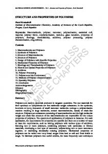
1. Introduction The atomic force microscope (AFM) is a major extension of scanning tunneling microscope (STM) and has borrowed some of the STM technology, including sub-nanometer motion and implementation of feedback technique. In AFM, the probe is a deflecting cantilever on which a sharp tip is mounted. As a topographic imaging technique, AFM may be viewed as a stylus profilimeter. Another major application of AFM is the measurement of the tip-sample interaction through force-distance curves. AFM force-distance curves have been used for the study of numerous material properties and for the characterization of surface forces. Especially, forcedistance curves are widely used for the determination of mechanical properties [1]. The elastic-plastic behavior and the hardness of a material are typically measured by its deformation response to an applied force. Microindentation probes to obtain this type of information have been employed for several years [1]. Recognizing the need to probe structures with considerably smaller dimensions at improved force and lateral resolution, there has been an effort to further reduce the area over which the measurement force is applied. The commercially available nanoindenters, which can resolve forces of 300 nN and depths of 0.4 nm, represent one step to satisfy these criterions [1]. The AFM provides orders of magnitude improvements over the nanoindenter, not only by superior performance in force and depth sensitivity for repulsive contact forces but also for use as an analogue to the surface force apparatus [1]. Since both attractive and repulsive forces localized over nanometer-scale regions can be probed, forces due to negative loading of the probe from the van der Waals attraction between tip and sample prior to contact, or from adhesive forces, which occur subsequent to contact, can be investigated. Over the last decade, the AFM has become one of the most important tools to study surface interaction by means of force-distance curves [2, 3]. In the past few years several scientific works have been aimed at determining the viscoelastic behavior and the glass transition temperature Tg through AFM measurements and most importantly using force-distance curves. In the first measurement using force-distance curves by Marti and his coworkers [4], the authors have observed a dramatic increase of adhesion above a certain temperature as shown in Fig. 1-1. The authors have acquired forcedistance curves on three PS samples having different molecular weights. The jump-offcontact was used to the measure of the tip-sample adhesion (see Section 3.2.1). The authors found out that the adhesion increases with increasing temperature and the increase of

1

Characterisation of Physical Properties of Polymers Using AFM Force-Distance Curves adhesion depends on the molecular weight of PS and therefore also on its Tg. The authors also showed that after cooling the samples the samples have the same tip-sample adhesion values at room temperature. See Section 2.6 for the dependence of Tg on the molecular weight of a polymer.

Figure 1-1: Adhesion of polystyrene having Mw = 2.5 (PS2.5), 6 (PS6) and 100 kg/mol (PS100) as a function of temperature measured by Marti et al. The adhesion increases at a certain temperature depending on the molecular weight. [Reproduced from Ref. 4] Later, Tsui and his coworkers have obtained force-distance curves at various temperatures on poly(t-butyl acrylate) [5]. The authors were able to draw a master curve of adhesion as shown in Fig. 1-2. The jump-off contact was used as the measure of tip-sample adhesion. The authors have also shown that there is a good agreement between the shift factors obtained using AFM and rheological measurements made on the bulk polymer.

Figure 1-2: Tsui et al. were able to draw a master curve of adhesion (markers) of poly(t-butyl acrylate) and compared the shift factors obtained using AFM and rheological measurements. [Reproduced from Ref. 5]

2

Introduction

Figure 1-3: The stiffness S, hysteresis H and pull-off force Fad measured from forcedisplacement curves obtained by Bliznyuk et al. as a function of temperature. The authors showed that these quantities change abruptly at T = Tg . [Reproduced from Ref. 6] Finally, Bliznyuk et al. [6] have measured several quantities from force-displacement curves acquired at different temperatures as shown in Fig. 1-3. The stiffness S of the sample is measured from the final gradient of the approach curve. A measure of the hysteresis H of the cycle is taken from the difference in displacement of the piezo on the approach and retraction at an arbitrarily fixed force of 0.1 µN. The authors have shown that both these quantities and the adhesion force change abruptly at the glass transition temperature. Unfortunately, these quantities have no physical meaning. Though this method provides a mean to evaluate Tg using AFM, it falls short of providing some insights into the physical processes occurring at T = Tg and into the dependency of physical quantities such as stiffness or hardness on

temperature and frequency. In order to determine the mechanical properties from force-distance curves, one of the elastic continuum contact theories, namely Hertz [7], Derjaugin-Müller-Toprov [8] and Johnson-Kendall-Roberts theory [9], has to be employed to know the dependence of the contact radius and the sample deformation on force. In his work, Maugis [10] combined the three major elastic continuum contact theories into a complete and general description, which showed the limits but most importantly the possibilities of AFM measurements of the elastic properties of materials. Quantitative determination of Young’s modulus has made good progress in the recent years [2, 3] and in several recent works, scientists have shown that quantitative determination of Young’s modulus of polymers and the comparison between the AFM data and the values reported using other techniques is possible [11-15].

3

Characterisation of Physical Properties of Polymers Using AFM Force-Distance Curves On the contrary, there are only very little important experimental results and theoretical studies on the plastic deformations of polymers to date [15]. However, yield strength and yielding behavior of polymers are of significance as they define the limits of load bearing capability of polymers with reversible deformations and also provide valuable insights into their modes of failure. In fact other established thermal analysis techniques such as dynamic mechanical analysis (DMA) can be used to measure the mechanical properties of polymers. However, measurements based on such techniques are performed on bulk polymer system whereas local measurements with very high lateral resolution in the order of nanometers are only possible with AFM measurements. Therefore, AFM force-distance curves provide an opportunity to measure differences in physical properties, e.g. stiffness or Tg, of heterogeneous samples such as polymer blends or copolymers. Polymer blends of homopolymers are interesting for diverse reasons and the properties of the polymer blends are largely determined by the morphology, i.e. the shape, size and distribution of the blend components. First, from a theoretical point of view, mixing of polymers is interesting as it is of great importance to know the structure and morphology of the polymer blend and the influence of the morphology on the resulting blend properties. Secondly, polymer blends allow the optimization of some properties compared to that of homopolymers. The interfacial properties between the two adjacent polymer phases are the least understood of all the properties of polymer blends. The limited amount of information available about the polymer-polymer interface is a direct consequence of the fact that very few techniques permit to study them directly [16, 17]. Several techniques are useful in studies of polymer interfaces, but they provide only indirect information [17-21]. Mapping the morphology and the composition of polymer blends and copolymers by means of AFM has made great stride in the last decade and it is an active field of research [18]. Some aspects of compositional identification are intrinsic to the AFM operation. The interaction forces acting between tip and sample surface comprise of chemical information, and the sample indentation contains details about the viscoelastic properties of the sample. Recently, AFM force-distance curves are gaining popularity to image contrast and to study the local variations of sample properties. Mechanical properties [13, 22] and the adhesion force [23-27] have been used to study the local variations of sample properties. However, in the past there have been no scientific studies of the temperature dependent mechanical properties of homogenous and heterogeneous polymer systems. 4

Introduction In the first part of the PhD work, the elastic-plastic behavior of poly(n-butyl methacrylate) is studied as a function of temperature and frequency. A novel analysis method based on Hertz theory [8], which also takes plastic deformations into account, has been used to determine the mechanical properties. Time-temperature superposition principle has been applied to the data obtained from the AFM measurements in order to present the results as a function of both temperature and frequency [28]. Similar measurements are carried out on two polystyrene samples having different Tg and molecular weight. The viscoelastic properties of the two polystyrene samples as a function of temperature are also studied [29]. Finally, force-distance curves are used to investigate a model polymer blend of polystyrene/poly(n-butyl methacrylate). The thermomechanical properties of the blend constituents in the vicinity of the interface and also far from the interface are compared to the measurements made on individual polymer films. Finally, the morphology of the blend is characterized as a function of temperature using the measured quantities [30]. In section 2, background information about the glass transition temperature and the viscoelastic behavior of polymers is presented. Section 3 deals with the working principle of AFM and especially, the force-distance curves and the elastic continuum theories to evaluate the mechanical properties. Sample preparation techniques, dynamical mechanical analysis and broadband spectroscopy measurements, and acquisition of force-distance curves are presented in Section 4. In Section 5, results from the measurements made on individual polymer films of poly(n-butyl methacrylate) and polystyrene are discussed and in Section 6, results from the measurements on a model polymer blend are presented.

5

Characterisation of Physical Properties of Polymers Using AFM Force-Distance Curves

2. Glass Transition Temperature and Viscoelastic Behavior of Polymers 2.1. The glass transition temperature Tg The glass transition is a phase change that occurs in solids, such as glasses, polymers and some metals. The glass transition temperature is defined as the temperature at which an amorphous material experiences a physical change from a hard and brittle condition to a flexible and rubbery condition. For polymers with both amorphous and crystalline regions (semicrystalline polymers) only the amorphous region exhibits a glass transition. The melting point Tm of crystalline solids or of the crystalline portion in semicrystalline polymers is the temperature at which they change their state from solid to liquid. Tm is a first order transition, i.e. volume and enthalpy (heat content) are discontinuous through the transition temperature. Unlike the melting point Tm, the glass transition temperature Tg is a second order transition, i.e. volume and enthalpy are continuous through the transition temperature. Since the glass transition phenomenon covers a wide range of temperatures without any discontinuity in the measured quantity at Tg, the reported Tg is generally taken as the mid-point of this range.

Figure 2-1: Volume-Temperature curves of a molten polymer (AE) forming a glassy amorphous state (EF) at the glass transition temperature Tg and of a liquid (AB) forming a crystalline solid phase (CD) at the melting point Tm. In the usual schedule schematically shown in Fig. 2-1, the solid is crystalline and passes into the liquid state at the melting point Tm. The transition is, in nearly all cases, accompanied by an increase in volume and in enthalpy, the latent heat of melting. The slope of the line DC is the thermal expansion coefficient of the crystalline phase and at the melting point the

6

Glass Transition Temperature and Viscoelastic Behavior of Polymers volume increases discontinuously from C to B. The slope of the line BA denotes the thermal expansion coefficient of the liquid phase, which is slightly higher than that of the crystalline solid phase. When the crystalline solid is cooled down, its volume retraces the path A to D. However, during cooling of an amorphous polymer from its melt, the polymer cools down along the line AB but from B to E it is in a flexible rubbery or leathery state, which solidifies at E without showing a discontinuous decrease in the volume. On further cooling, the polymer undergoes a transformation into a glassy amorphous state, with about the same thermal expansion coefficient of the crystalline counterpart. For an amorphous polymer, the temperature at which the slope of the volume-temperature measurement changes is referred as the glass transition temperature Tg. When a polymer is heated up above its Tg, it is not immediately transformed into its molten state, but first into a rubbery state which gradually melts upon further heating. Therefore, Tg is also called the glass-rubber transition temperature. It is appropriate to point out that the Tg value recorded in any given experiment is dependent on the temperature-scanning rate or on the frequency [31, 32]. This is further discussed in Section 2.5. In the glassy state the molecular structure is highly disordered. This is clearly demonstrated by X-ray diffraction patterns in the glassy state, where only a diffuse ring is visible, indicating some short-distance order. In contrast, sharp reflections are obtained for crystalline materials which exhibit long-range order. The disordered glassy state occupies a larger volume than a crystal and this excess volume due to the lack of ordering in the system is called the free volume Vf. This is the reason for the difference between the volume of an amorphous polymer below Tg (line EF) and the volume of a crystalline counterpart (line CD) in Fig. 2-1. In order to calculate the total free volume, we only need to know the density of the material and the radii of the atoms. However, the free volume that is accessible to the atoms is far less than the total free volume and it depends on the size of the moving atom or group of atoms. The reminder of this chapter presents information about the free volume concept and the relaxation time of transitions, the viscoelastic behavior of polymers, the time-temperature superposition principle, sub-Tg relaxations, non-equilibrium phenomena in glass transition and the effect of molecular structure on Tg.

2.1.1. Free volume concept The thermal transitions in polymers can be described in terms of either free volume changes or relaxation times. A simple approach to the concept of free volume, which is

7

Characterisation of Physical Properties of Polymers Using AFM Force-Distance Curves popular in explaining the dynamic mechanical properties, is the crankshaft mechanism, where the molecule is imagined as a series of jointed segments. Taking advantage of this model, it is possible to simply describe the various transitions seen in polymers. Other models exist that allow for more precision in describing polymer behavior; the best seems to be the DoiEdwards model [33].

Figure 2-2: The crankshaft model showing the possible movements involving side groups and main chains as a result of increase in free volume on heating a polymer. The movements can involve stretching, bending and rotation of side groups or coordinated movements and chain slippage involving main chains. The crankshaft model treats the polymer chains as a collection of mobile segments that have some degree of free movement, as shown in Fig. 2-2. This is a very simplistic approach, yet very useful for explaining the polymer behavior. When the free volume accessible to the movement of atoms is small ( T < Tg ), segments of main chain or side group elements can rotate or stretch around their axes without changes in the bond angle or can bend with small changes in the bond angles. When the free volume is largely increased ( T > Tg ), segments of one main chain can move in a coordinated fashion with segments of another main chain or whole polymer chains can slip past one another. When a polymer is heated up, the free volume of the chain segment increases and the ability of the chain segments to move in various directions also increases. This increased mobility in either side chains or small groups of adjacent backbone atoms results in various

8

Glass Transition Temperature and Viscoelastic Behavior of Polymers transitions affecting several properties of the polymer, e.g. mechanical and dielectric properties. Figure 2-3 schematically shows the effect of these transitions on the modulus E of the polymer as a function of temperature and the chain conformations associated with each transition according to the crankshaft model. As the polymer heats up and expands, the free volume increases so that localized bond movements (rotating, bending and stretching) and side chain movements can occur. This is the gamma transition at Tγ. As the temperature and the free volume continue to increase, the whole side chains and localized groups of 4-8 backbone atoms begin to have enough space to move and the material starts to develop some toughness. This transition is called the β transition (see Section 2.3). Often it is the Tg of a secondary component in a blend or of a specific block in a block copolymer.

Figure 2-3: A schematic representation of the effect of temperature on the modulus E of an amorphous polymer and the corresponding chain conformations (numbers 1-6) associated with each transition region. The sub-Tg β and γ transitions occur at Tβ and Tγ.

As the free volume continues to increase with increasing temperature, the glass transition Tg occurs when large segments of the chains start moving. In most polymers, there is almost

three orders of magnitude decrease in the Young’s modulus E of the polymer at Tg. The plateau between the glass-rubber transition region and the melt region is known as the rubbery plateau. Large scale main chain movements occur in the rubbery plateau and the modulus remains fairly constant exhibiting highly elastic properties. On continued heating, the melting point, Tm, is reached. The melting point is where the free volume has increased so that the

9

Characterisation of Physical Properties of Polymers Using AFM Force-Distance Curves chains can slide past each other and the material flows. This is also called the terminal region. In the molten state, the ability to flow is dependent on the molecular weight of the polymer.

2.1.2. Relaxation time On a molecular scale, when a polymer is at T = 0 K, the chains are at absolute rest. No thermal motions occur and everything is completely frozen in. When the temperature is increased, the thermal motions increase and gradually short parts of the chain or side groups may obtain some mobility, which, within the restricted free volume, gives rise to small changes in conformation. Whether this occurs or not is a matter of competition between the thermal energy of a group (kBT) and its interaction with neighboring groups. The interaction can be expressed as a potential barrier or activation energy Ea which has to be overcome in order to realize a change in position. As the temperature increases, the fraction of groups able to overcome the potential barrier increases. The jump frequency ν with which the changes occur can be expressed by the Arrhenius equationν = ν 0 exp(− E a k BT ) , where ν0 is the natural frequency of vibration about the equilibrium position and kB is the Boltzmann constant. The jump frequency governs the time scale τ at which the transition occurs. τ is inversely proportional to ν:

τ = A exp(E a k BT ) ⇒ ln τ = ln A +

Ea . k BT

(2.1)

This equation provides a fundamental relationship between the effects of time and temperature on a transition mechanism. Time and temperature appear to be equivalent in their effect on the behavior of polymers.

2.1.3. Thermodynamics of the glass-rubber transition To consider the nature of glass-rubber transition on a thermodynamic basis, we should first compare it with melting. The melting point is a first-order transition but glass transition partially obeys second-order characteristics. The quantity G, the Gibbs free energy, plays a predominant role in the thermodynamic treatment of transitions. G = U − TS + pV = H − TS = A + pV .

(2.2)

Here, U is the internal energy (result of the attractive forces between molecules), T is the absolute temperature, S is the entropy (measure of disorder in the system), p is the pressure, V is the volume, H is the enthalpy or the heat content of the system and A is the Helmholtz free energy.

10

Glass Transition Temperature and Viscoelastic Behavior of Polymers With each type of transition, ∆G = 0, or, in other words, the G(T) curves for both phases intersect, and slightly below and above the transition temperature the Gibb’s free energy is the same. The various derivatives of the free enthalpy may however show discontinuities. For a first-order transition such as melting, the first derivatives like V, S and H are discontinuous at the melting point Tm. On the contrary, the glass-rubber transition does not show discontinuities in V, S and H as illustrated in Fig. 2-4a. However, discontinuities occur in the derivatives of these quantities, such as thermal expansion coefficient (α = dV/dT), specific heat capacity (Cp = dH/dT) and compressibility:  ∂G   ∂p  = V , Vglass = Vrubber , ∆V = 0 .  T

(2.3)

 ∂ 2 G   ∂V    =   = αV , α glass ≠ α rubber . ∂ p ∂ T    ∂T  p

(2.4)

There are discontinuities in the second derivatives of the free enthalpy G, and, for this reason, the glass-rubber transition is denoted as a second-order transition. Figure 2-4b shows the discontinuity in thermal expansion coefficient or the heat capacity of an amorphous polymer in the glass-rubber transition region. Tg can be determined either from the onset or from the midpoint of the transition region, where the onset point is the intersection of the initial region straight line and the transition region straight line (red lines) as illustrated in Fig. 2-4b.

Figure 2-4: (a) Continuous functions of volume V or enthalpy H at Tg. (b) Thermal expansion coefficient dV/dT or specific heat capacity dH/dT exhibit discontinuities at Tg as glass-rubber transition follows second-order transition characteristics. The onset is the intersection of the initial region straight line and the transition region straight line (red lines).

11

Characterisation of Physical Properties of Polymers Using AFM Force-Distance Curves In case of glass-rubber transition, a state of thermodynamic equilibrium is not reached and the measured Tg is probe rate dependent (see Section 2.5). Hence, glass transition is not a strict second-order transition.

2.2. Viscoelastic properties of polymers A viscoelastic material is one which shows hysteresis in stress-strain curve, creep (increasing strain for a constant stress) and stress relaxation (decreasing stress for a constant strain). Almost all polymers exhibit viscoelastic behavior. Polymers behave more like solids at low temperatures ( T < Tg ) and/or fast deformation rates and they exhibit more liquid like behavior at high temperatures ( T > Tg ) and/or slow deformation rates. It is also necessary to emphasize that even in the glassy or molten state, the response is partly elastic and partly viscous in nature. As a common practice, a system that reacts elastically or viscously is represented by a spring or dashpot model obeying Hooke’s or Newton’s law. Maxwell element combines a spring and a dashpot in series and Kelvin-Voigt element combines them in parallel. Various combinations of Maxwell or Kelvin-Voigt mechanical model elements in series or parallel configurations have been used in an attempt to describe the viscoelastic behavior of polymers.

2.2.1. Dynamic mechanical properties Dynamic mechanical properties refer to the response of a material as it is subjected to a periodic force. These properties may be expressed in terms of a dynamic modulus, a dynamic loss modulus, and a mechanical damping term. Values of dynamic moduli for polymers range from 0.1 MPa to 100 GPa depending upon the type of polymer, temperature, and frequency. Typically the Young’s modulus of an amorphous polymer in its glassy state is in order of few GPa. For an applied stress varying sinusoidally with time, a viscoelastic material will also respond with a sinusoidal strain for low amplitudes of stress. The strain of a viscoelastic body is out of phase with the stress applied by the phase angle δ as shown in Fig. 2-5. This phase lag is due to the excess time necessary for molecular motions and relaxations to occur. Dynamic stress σ and strain ε are given as:

12

σ = σ 0 sin (ωt + δ ) ⇒ σ = σ 0 sin (ωt ) cos δ + σ 0 cos(ωt ) sin δ

(2.5)

ε = ε 0 sin (ωt )

(2.6)

Glass Transition Temperature and Viscoelastic Behavior of Polymers

Figure 2-5: The phase lag δ between the applied stress σ (red) and the resulting strain ε (blue) due to the viscoelastic nature of a polymer. where ω is the angular frequency. Using this notation, stress can be divided into an “in-phase” component and an “out-of-phase” component. Dividing stress by strain to yield a modulus and using the symbols E ' and E" for the in-phase (real) and out-of-phase (imaginary) moduli yields: σ0   E ' = ε cos δ  0   E" = σ 0 sin δ  ε0

(2.7)

σ = ε 0 E ' sin (ωt ) + ε 0 E" cos(ωt )

(2.8)

E* =

σ σ0 (cos δ + i sin δ) = E '+iE" = ε ε0

tan δ =

E" E'

(2.9)

(2.10)

The real (storage) part describes the ability of the material to store potential energy and release it upon deformation. The imaginary (loss) portion is associated with energy dissipation in the form of heat upon deformation and tan δ is a measure of the mechanical damping. The above equation can be rewritten for shear modulus G * as, G * = G '+iG"

(2.11)

where G ' is the shear storage modulus and G" is the shear loss modulus, and the phase angle δ is:

13


tan δ =

G" . G'

(2.12)

The storage modulus is related to the stiffness and the Young’s modulus E of the material. The dynamic loss modulus is associated with internal friction and is sensitive to different kinds of molecular motions, relaxation processes, transitions, morphology and other structural heterogeneities. The storage modulus, the loss modulus and tan δ as a function of temperature are illustrated in Fig. 2-6. Here, one can see that with the onset of glass transition, the mechanical damping coefficient tan δ, increases and reaches its peak. Also, the loss modulus increases and reaches a peak value in the glass transition window, where the storage modulus decreases sharply. Thus, the dynamic properties provide information at the molecular level to understand the mechanical behavior of polymers.

Figure 2-6: Illustration of the storage modulus E’ (blue circles), the loss modulus E” (green squares) and the mechanical damping coefficient tan δ (black triangles) of poly(n-butyl methacrylate) as a function of temperature. The loss modulus and the mechanical damping coefficient reach their peak value within the glass-rubber transition window, where the storage modulus decreases sharply. Five different values can be described as Tg from these curves. They are the peak or onset of the tan δ curve, the onset of decrease in the E ' curve, or the onset or peak of the E" curve. The onset is the intersection of the initial region straight line with the transition region straight line (blue and black lines for E ' and tan δ, respectively). The onset point of E" is not shown here because of the strong β relaxation occurring close to Tg (see Section 2.3).

14

Glass Transition Temperature and Viscoelastic Behavior of Polymers

2.2.2. Time-temperature superposition principle Time-temperature superposition principle TTS can be used to detect the glass transition temperature of polymers due to the viscoelastic nature of polymers. TTS, or temperaturefrequency superposition, the equivalent, was at first experimentally noticed in the late 1930s in a study of viscoelastic behavior in polymers and polymer fluids [33]. Afterwards, further studies indicated that the TTS could be explained theoretically by some molecular structure models [33]. A dynamic property of polymer (e.g. storage modulus) is influenced by the temperature and the frequency (or the response time) of the dynamic loading. According to the principle of TTS, the frequency function of E at a given temperature T0, is similar in shape to the same functions at the neighboring temperatures. Hence it is possible to shift the curves along the horizontal direction (in terms of frequency or time) so that the curve overlaps the reference curve obtained at reference temperature either partially or fully depending on the temperature interval as demonstrated in Fig. 2-7. Here the reference temperature is chosen as -83 °C. After shifting the curves, the frequency range of the experiment has increased by many orders of magnitude. The shift distance along the logarithmic frequency axis is called the frequency-temperature shift factor aT and is:

aT =

f0 fT

(2.13)

where fT is the frequency at which the material reaches a particular response at temperature T and f0 is the frequency at which the material achieves the same response at the reference temperature T0. For the overlapped portion of the curve: E (T , a T f ) = E (T0 , f ) .

(2.14)

The value of the shift distance is dependent on the reference temperature and the material properties of the polymers. For every reference temperature chosen, a fully overlapped curve can be formed. The overlapped curve is called the master curve. The shift factors of a master curve have experimentally some relationship with the temperature. Since 1950s, dozens of formulae have been proposed to link the shift factors of a master curve to temperature. One of the most recognized formulae was established in 1955 and is known as Williams-LandelFerry or the WLF equation [36]. For the temperature range above Tg, it is generally accepted that the shift factor-temperature relationship is best described by the WLF equation:

log aT =

− C1 (T − T0 ) , C 2 + (T − T0 )

(2.15)

15

Characterisation of Physical Properties of Polymers Using AFM Force-Distance Curves where C1 and C2 are constants. If T0 is taken as Tg, for a temperature range of Tg to Tg + 100 °C, a set of ‘universal constants’ for the WLF coefficients are considered reliable for

the rubbery amorphous polymers. Their values are C1 = 17.44 and C 2 = 51.6 °C .

Figure 2-7: Time-temperature superposition principle applied to isotherms of the storage modulus E ' obtained on an amorphous polymer at -83, -79, -77, -74, -71, -66, -62, -59, -50, and -40 °C and at various frequencies on the left hand side of the image. The reference isotherm is -83 °C and all the other isotherms are shifted in order to overlap the reference curve either fully or partially forming the master curve of the storage modulus on the right hand side of the image for a wide range of frequency.

The WLF equation in terms of aT has been rationalized using Doolittle’s free volume theory [37]. According to this theory that portion of the volume which is accessible to the kinetic process of interest is considered to be the free volume Vf = V − V0 , where V is the measured volume and the inaccessible volume V0 is called the occupied volume. The Doolittle equation states that the viscosity η is an exponential function of the reciprocal of the relative free volume: φ = Vf / V0 ,

η = Ae

b

φ

,

(2.16) (2.17)

where A and b are empirical constants, the latter of the order of unity. In WLF equation, the fractional free volume f = Vf V was chosen in place of φ. This substitution made no

16

Glass Transition Temperature and Viscoelastic Behavior of Polymers difference in the derivation of the equation for the temperature shift factor aT and they obtained

log aT =

(b 2.303 f 0 )(T − T0 ) f 0 α f + T − T0

.

(2.18)

Eq. 2.18 is identical in form with the WLF equation with C1 = (b 2.303 f 0 ) and C 2 = f 0 α f , where f0 is the initial free volume and αf is the thermal expansion coefficient of fractional free volume. For the temperature range below the glass transition temperature, the Arrhenius equation is generally acknowledged as the suitable equation to describe the relationship between the shift factors of the master curve and the reference temperature as

ln aT =

Ea R

1 1   −  + ln A ,  T T0 

(2.19)

where Ea is the activation energy of the relaxation process and R is the universal gas constant (8.3144 × 10-3 kJ/mol K). Here, the activation energy associated with the transitions in a polymer can be estimated from the plot of the shift factors vs. the logarithm of frequency. The intersection of the Arrhenius equation with the WLF equation for the shift factors of the master curve can be used to estimate Tg of a polymer provided the reference temperature T0 is chosen close to Tg.

2.3. Sub-Tg relaxations in polymers Besides the glass-rubber transition, amorphous polymers show also one or more sub-Tg processes, which are referred to as β, γ, and δ transition as they appear in order of descending temperature. The sub-Tg processes are the result of local segmental motions occurring in the glassy state. By ‘local’ is meant that only a small group of atoms are involved in the process. The pure existence of these processes proves that the glassy material is a dynamic material. The experimental evidence for the sub-Tg processes originated from dynamic mechanical analysis (DMA), dielectric or broadband spectroscopy and nuclear magnetic resonance spectroscopy (NMR). Figure 2-8 shows the influence of the sub-Tg relaxation processes on the quantity tan δ (Eq. 2.10) as a function of temperature. The molecular interpretation of the sub-Tg processes has been the subject of considerable interest from the later half of the last century. By varying the repeating unit structure and by studying the associated relaxation processes, it has been possible to make a group assignment of the relaxation processes. That is not to say that the actual mechanism has been resolved.

17

Characterisation of Physical Properties of Polymers Using AFM Force-Distance Curves The relaxation processes can be categorized as side-chain or main-chain relaxation. Sub-Tg processes appear both in polymers with pendant groups such as poly(methyl methacrylate) and in linear polymers such as polyethylene or poly(ethylene terephthalate). In the latter case, the sub-Tg process must involve motions in the backbone chain. Sub-Tg transitions also show frequency dependence like glass-rubber transition temperature, although its activation energy is only 30-40 J/g.

Figure 2-8: Typical tan δ of an amorphous polymer as a function of temperature showing the sub-Tg β and γ relaxations at Tβ and Tγ below Tg. The magnitude of the mechanical damping at Tg is much larger when compared to the other sub-Tg transitions.

The field of sub-Tg or higher order transitions has been heavily studied as these transitions have been associated with mechanical properties in glassy state. Sub-Tg transitions can be considered as the “activation barrier” for solid phase reactions, deformation, flow or creep, acoustic damping, physical aging changes, and gas diffusion into polymers as the activation energies for the transition and these processes are usually similar [34]. The strength of the β transition is taken as a measurement of how effectively a polymer will absorb vibrations. A working rule of thumb is that the β transition must be related to either localized movement in the main chain or very large side chain movement to sufficiently absorb enough energy as β transition is generally associated with the toughness of polymers. Boyer and Heijober showed that this information needs to be considered with care as not all β transitions correlate with toughness or other properties [38, 39]. The γ transition is mainly studied to understand the movements occurring in side chain polymers. Schartel and Wendorff reported that this transition in polyarylates is limited to

18

Glass Transition Temperature and Viscoelastic Behavior of Polymers inter- and intramolecular motions within the scale of a single repeat unit [40]. McCrum similarly limited the Tγ and Tδ to very small motions within the molecule [41]. In brief, the relaxation processes taking place in poly(n-butyl methacrylate) (PnBMA) and polystyrene (PS) will be discussed as these are the two polymers that have been studied in this work. The molecular structures of PnBMA and PS are shown in Fig. 2-9. Polystyrene exhibits relatively complex relaxation behavior. Apart from the glass transition, polystyrene exhibits three sub-Tg relaxation processes. One view is that the cryogenic δ process at -218 °C and 10 kHz is due to oscillatory motions of the phenyl groups, whereas Yano and Wada believe that the δ relaxation process arises from defects associated with the configuration of the polymer [42]. The γ process appearing at -93 °C and 10 kHz has also been attributed to phenyl group oscillations or rotations. The high temperature β relaxation process occurs around 52 °C and is believed to be due to the rotation of the phenyl groups with main chain cooperation and the activation energy Ea associated with the transition is 147 kJ/mol [43].

Figure 2-9: The molecular structure of poly(n-butyl methacrylate) and polystyrene. In PnBMA, the predominant sub-Tg relaxation process is the strong β relaxation occurring around its Tg (22 °C). The β relaxation process shows both mechanical and dielectric activity and it is assigned to rotation of the butyl side group. Since the β relaxation occurs close to Tg, it is difficult to measure the effect of the β relaxation on the mechanical properties of the polymer. The dipole moment is located in the side group − COO − (CH 2 ) 3 − CH 3 , hence it can contribute significantly to the dielectric loss. Peculiarities in the relaxation behavior of this class of polymers might also be the reason for the unusual value of the C2 coefficient [44]. To this date the exact reason for such a behavior is unclear. A low temperature (-140 °C) γ relaxation, following Arrhenius temperature-dependence, occurs in side chain polymers with

19

Characterisation of Physical Properties of Polymers Using AFM Force-Distance Curves at least four methylene groups. This low temperature process was attributed to restricted motion (crankshaft mechanism) of the methylene sequence [34].

2.4. Determination of glass transition temperature For amorphous polymers, the glass transition temperature can be determined using standardized methods such as: specific volume measurement, differential scanning calorimetry (DSC), thermomechanical analysis (TMA), dynamic mechanical analysis (DMA) or dynamic mechanical thermal analysis (DMTA) and broadband or dielectric spectroscopy at a fixed heating or cooling rate. In specific volume measurements, the changes in the dimension (specific volume) of the sample are determined as a function of temperature and/or time as shown in Fig. 2-1. At Tg, the specific volume discontinuously increases from the glassy state to the rubbery state. The intersection of the initial straight line and the transition region straight line of the specific volume vs. temperature curve is designated as Tg. The dielectric function of the polymer is measured in broadband spectroscopy and the dielectric function varies significantly when transitions or relaxations occur in polymers. Broadband spectroscopy is mostly used in studying the sub-Tg transitions in polymers as it is very sensitive to small changes occurring in dielectric properties during sub-Tg transitions. In DSC, the difference in the amount of heat required to increase the temperature of a sample and reference are measured as a function of temperature. Both the sample and reference are maintained at the same temperature throughout the experiment. Generally, the temperature program for a DSC analysis is designed such that the sample holder temperature increases linearly as a function of time. The reference sample has a well-defined heat capacity over the range of temperatures to be scanned. The basic principle underlying this technique is that, when the sample undergoes a physical transformation such as a phase transition, more (or less) heat will need to flow to it than the reference to maintain both at the same temperature as shown below in Fig. 2-10. Whether more or less heat must flow to the sample depends on whether the process is exothermic or endothermic. For example, as a solid sample melts to a liquid it will require more heat flowing to the sample to increase its temperature at the same rate as the reference. This is due to the absorption of heat by the sample as it undergoes the endothermic phase transition from solid to liquid (also from glassy to rubbery). Likewise, as the sample undergoes exothermic processes (such as crystallization) less heat is required to raise the sample temperature. By observing the difference in heat flow between the sample and reference, differential scanning calorimeters are able to measure the amount of

20

Glass Transition Temperature and Viscoelastic Behavior of Polymers energy absorbed or released during such transitions. Due to the difference between the heat capacities of the polymer in glassy and rubbery state, a small step is seen in the heat flow during glass-rubber transition.

Figure 2-10: Heat flow as a function of temperature of a semicrystalline polymer measured using DSC. The curve shows the endothermic glass-rubber transition, the exothermic crystallization process and the endothermic melting process. Tg of the amorphous region, the crystallization temperature Tc and the melting temperature Tm can be measured using DSC curves.

In DMA, the polymer is subjected to periodic stress and the resulting periodic strain (outof-phase) is measured as a function of temperature. During a single scan, it is possible to apply a wide range of periodic stresses with DMA, whereas in TMA the stress can be applied only at one frequency. The modulus is obtained from the stress-strain relationship and the complex modulus comprises of E ' (elastic property) and E" (viscous property). The ratio between loss E" and storage E ' moduli gives the mechanical damping coefficient tan δ. Figure 2-6 shows the 4 possible temperatures that could be mentioned as Tg in DMA measurements. The blue, green and grey lines are used to determine the onset on the storage modulus (blue circles), loss modulus (green squares) and tan δ (black triangles) curves respectively. The peak or onset of increase in the tan δ curve, the onset of decrease in E ' , or the onset of increase in E" or its peak may be used as recorded Tg values. The strong influence of the β transition on the loss modulus close to Tg makes it difficult to unambiguously determine the onset of increase in the loss modulus for this polymer. Hence, the onset of decrease in E" is not shown here. The values obtained from these methods can differ up to 25 °C from each other on the same run. In practice, it is important to specify exactly how the Tg has been determined. It is not unusual to see a peak or hump on the storage 21

Characterisation of Physical Properties of Polymers Using AFM Force-Distance Curves modulus E ' directly preceding the drop that corresponds to the Tg. This is also seen in the DSC and other DTA methods and it corresponds to the rearrangement in the material to relieve stresses induced by the processing method. These stresses are trapped in the material until enough mobility is obtained at Tg to allow the chains to move to a lower energy state. Often a material will be annealed by heating it above Tg and slowly cooling it to remove this effect. For similar reasons, some experimenters will run a material twice or use a heat-coolheat cycle to eliminate processing effects. It is important to remember that the Tg has a pronounced sensitivity to frequency, shifting even sometimes about 5-7 degrees for every decade change in frequency. Measuring the activation energy associated with a transition and finding it to be about 300-400 J/g is one way to assure the measured transition is really the glass-rubber transition. As mentioned already, the glass transition can be considered as a second order phase change, which means that the changes in specific volume and heat capacity through the transition interval are continuous making determination of Tg not a straight forward task. In the cases of composites, semicrystalline polymers and polymers with wide molecular mass distribution, the onset point on the curves of specific volume measurements or any of the differential thermal methods is difficult to define unequivocally. Therefore, the task of determining Tg is not straight forward and it is important to state the technique and the parameters used.

2.5. Physical aging and cooling rate dependency of Tg The glass transition partially obeys second order characteristics, i.e. volume and enthalpy are continuous through the transition temperature. However, their temperature derivatives, the thermal expansion coefficient and the specific heat, show discontinuity at the glass transition temperature. The experiment schematically represented by Fig. 2-11 shows the nonequilibrium nature of a polymer that has been cooled at a constant rate q through the kinetic glass transition region. The volume may be continuously measured in a dilatometer. The sample is first heated to a temperature well above Tg (point A). Then the sample is cooled at a constant rate q. At point B the volume decrease is retarded. A change in the slope of the curve occurs at the glass transition temperature Tg(q), which is interpreted as being the kinetic glass transition. At C, a few degrees below B, the cooling is stopped and the sample is held at that temperature. The volume of the material decreases under isothermal conditions as a function of time, following the line CD, showing that equilibrium has not been attained at point C. It may be argued that equilibrium has not been reached in any of the points between B and C,

22

Glass Transition Temperature and Viscoelastic Behavior of Polymers i.e. the recorded glass transition has kinetic features. The process transferring the system from C towards D is denoted as physical aging or simply in this case isothermal volume recovery.

Figure 2-11: Volume-Temperature curve of a molten polymer (AB) forming a glassy amorphous state (BC) on cooling at a constant rate q at the glass transition temperature Tg(q). The volume decreases from C to D when the cooling is stopped. The process transferring the polymer system from C towards D is known as isothermal volume recovery or physical aging.

The term recovery is often used instead of relaxation to indicate that the process leads to the establishment (recovery) of equilibrium. The volume may be replaced by enthalpy, and curves similar to that shown in Fig. 2-11 are obtained. The approach of the non-equilibrium glass to the equilibrium state is accompanied by a decrease in enthalpy (isothermal enthalpy recovery), which can be detected in-situ by a differential scanning calorimeter (DSC). Even if such equilibrium would exist, it would be at a much lower temperature. On the basis of theoretical calculations, it has been supposed that a real second-order transition could occur at a temperature 50 to 60 °C below the observed value of Tg [35]. This temperature would be reached after extremely low rates of cooling. Even at 70 °C below Tg no indication of a transition was found [35]. Estimations on the basis of empirically found relation between Tg and the rate of cooling indicate that the required time would be of the order of 1017 years [35]. Thus, it appears that the glass transition, even with infinitely low cooling rate, is not a real thermodynamic transition, but only governed by kinetics as a freezing-in phenomenon.

23


Figure 2-12: Young’s modulus of PnBMA obtained as a function of temperature at 50 Hz (red filled squares), 30 Hz (blue empty circles), 1 Hz (black filled squares) and 0.3 Hz (green empty circles) using dynamic mechanical analysis. The measured Tg increases with increasing frequency. This measurement has been performed in collaboration with Dr. Wolfgang Stark at the Bundesanstalt für Materialforschung –und Prüfung, Berlin.

Figure 2-12 shows the response of Young’s modulus of an amorphous polymer as a function of temperature measured at various frequencies. One can point out that the recorded Tg increases with increasing frequency from 0.3 Hz to 50 Hz. At 0.3 Hz the Tg of polymer is

20.4 °C and Tg increases to 27 °C when the frequency is increased to 50 Hz. As mentioned earlier, one can see that, at higher frequencies, the time available to the system to relax is at each temperature shorter than at a lower frequency. This reflects a decrease in the molecular mobility at higher frequencies as the time available for relaxation is less, which leads to an increase in the recorded glass transition temperature. Experimental work has shown that Tg is changed by approximately 3 °C if the frequency is changed by a factor of ten [31, 32]. In some polymers, Tg varies by 5-7 °C for a decade change in the frequency.

2.6. Dependence of Tg on molecular architecture Glass transition temperature largely depends on the chemical structure and molecular mobility of materials. Molecular weight, stiffness of the molecular chain, intermolecular forces, cross-linking and side chain branching all have effects on molecular mobility, therefore also on the glass transition temperature [31].

24

Glass Transition Temperature and Viscoelastic Behavior of Polymers The variation in glass transition temperature of a homopolymer due to changes in molar mass M is significant. With each chain end a certain degree of extra mobility is associated. A certain excess free volume ∆Ve may be assigned to each chain end. For each polymer chain, the excess free volume becomes 2∆Ve resulting from the two chain ends. The excess volume per unit mass is 2∆Ve NA/M, where NA is the Avogadro number. The excess free volume per unit volume fe of the polymer is obtained by multiplying with the density ρ

fe =

2ρ∆Ve N A . M

(2.20)

The free volume theory states that any fully amorphous material at the glass transition temperature takes a certain universal fractional free volume denoted fg. At the glass transition temperature of a polymer with infinite molar mass Tg∞ , the fractional free volume of the polymer with molar mass M is equal to:

f = fg +

2ρ∆Ve N A . M

(2.21)

This free volume can also be expressed as the sum of the universal free volume at Tg(M) for the polymer with molar mass M and the thermal expansion from this temperature to Tg∞ as

{

}

f = f g + α f Tg∞ − Tg (M ) ,

(2.22)

where αf is the thermal expansion coefficient of the fractional free volume. By combining Eqs. 2.21 and 2.22, the following expression is obtained.

Tg (M ) = Tg∞ −

2ρ∆Ve N A K ⇒ Tg (M ) = Tg∞ − αf M M

(2.23)

Eq. 2.23 was first suggested by Fox and Flory [45]. The excess free volume (∆Ve) can be obtained from the slope coefficient in a Tg vs. 1/M plot. Values in the range 20 to 50 Å3 have been reported [32]. The molar mass M in Eq. 2.23 should be replaced by the number average molecular mass Mn for polydisperse polymers.

25


3. Atomic Force Microscope (AFM) In 1981, the invention of scanning tunneling microscope (STM) by Binnig et al. [46, 47] transformed the field of microscopy. For the first time images of conducting and semiconducting materials with atomic scale resolution were reported. This led to a series of scanning probe microscope (SPM) inventions in the 1980s. STM was followed in 1984 by scanning near-field optical microscope (SNOM), which allowed microscopy with light below the optical resolution limit [48, 49]. In 1986, Binnig et al. [50] invented the atomic force microscope (AFM). Instrumental improvements and novel applications of AFM have broadened rapidly in the last two decades, so that AFM has become the most useful tool to study local surface interactions by means of force-distance curves [2, 3] and the most important SPM together with its “daughter” instruments, such as magnetic force microscope and Kelvin probe microscope [51, 52]. SPM images the sample surfaces using a physical probe (a sharp tip) by moving the sample in a raster scan and recording the tip-sample force as a function of position. In contrast to STM, which senses the tunneling current between the conducting tip and specimen, AFM, probing tip-sample forces can be used also with non-conducting materials, e.g. polymers and biological samples [2, 3]. Forces of the order of 10-12 to 10-4 N can be measured with a lateral resolution of the order of Angstroms [53]. From the beginning it was evident that the AFM was not only able to image the sample topography but also to detect a variety of different forces. In addition to ionic repulsion forces, also van der Waals, magnetic, electrostatic and frictional forces could be readily measured by AFM [2, 3]. Several other methods can be used to study the surface interactions and one of the most popular among them is the surface force apparatus (SFA) [54]. SFA has a vertical resolution of 0.1 nm and a force resolution of 10 nN. SFA employs only surfaces of known geometry (two curved molecularly smooth surfaces of mica), thus leading to precise measurements of surface forces and energies [2]. However, only a limited number of systems could be investigated because of the complexity of the instrument and the restrictions imposed on the material properties. The major drawback of SFA is that it cannot be used to scan the surface of the sample, so that no topography can be acquired. Besides, AFM offers more versatility than SFA because AFM measurements can work with smaller interacting surfaces (104 to 106 times smaller), with opaque substrates, in several environments, and can be used to characterize indentations [2]. Due to its high lateral resolution AFM can be also used for

26

Atomic Force Microscope (AFM) mapping inhomogeneities in small samples or variations in sample properties over the scanned area.

3.1 Fundamental principles of AFM AFM is a local probe technique, designed to measure interaction forces between a sharp tip and the sample surface. The working of an atomic force microscope is schematically represented in Fig. 3-1. The heart of AFM is a cantilever with a sharp microfabricated tip, whose edge radius is in the order of nanometers. The tip is attached to one end of the cantilever and the other end of the cantilever is fixed to a solid support (chip). In order to acquire the topography or the interaction forces on each point of the sample, the sample must be moved in a raster scan for several micrometers with a high lateral resolution (1 Å). To this aim the sample is mounted on a piezoscanner that can move the sample in x, y, and z directions. A laser beam is focused on to the back surface of the cantilever and the cantilever reflects the laser on to a segmented photodiode. On interacting with the sample the cantilever deflects and the laser spot on the photodiode moves proportional to the cantilever deflection. A feedback mechanism keeps constant the tip-sample distance by adjusting the measured quantity (deflection or oscillation amplitude, depending on the operation mode), and so preventing the tip and sample from being damaged. A controller is used to collect and process the data, and to drive the piezoscanner.

Figure 3-1: Schematic of an atomic force microscope (AFM). The sample is mounted on a piezo scanner capable of performing small displacements in the x, y, and z directions. The cantilever deflection caused by the tip-sample interaction is detected using the laser beam reflected on to a photodiode. A controller is used to collect and process the data and to drive the piezoscanner. 27

Characterization of Physical Properties of Polymers Using AFM Force-Distance Curves AFM can be operated in a variety of environments such as air, different gases, vacuum or liquids. Nowadays, commercially available AFM are equipped with environmental cells in which the temperature and the environment can be controlled.

3.1.1. Modes of operation AFM can be operated in various modes to measure the interaction forces as a function of the tip position over the entire scanned area. These modes differ according to the force between the tip and sample. The first and foremost mode of operation is contact mode. As the tip is raster-scanned across the surface, it is deflected as it moves over the surface corrugation as shown in Fig. 3-2a. In constant force mode, the tip is constantly adjusted using the feedback mechanism to maintain a constant deflection, and therefore constant height above the surface. The changes in the feedback signal required to maintain the force constant are used to reconstruct the topography. However, the ability to track the surface in this manner is limited by the feedback circuit. Sometimes the tip is allowed to scan without this adjustment, and one measures only the deflection. This is useful for small, high-speed atomic resolution scans, and is known as variable-deflection mode. As the tip is in hard contact with the surface, the stiffness of the cantilever needs to be less that the effective spring constant holding atoms together, which is on the order of 1-10 nN/nm. Most contact mode levers have a spring constant of dFsurf dD , the total force F increases for a small movement of the tip. The positive restoring force drives the tip back to its previous position but when the net force is negative, i.e. k c < dFsurf / dD , the tip is driven further towards the sample surface and eventually the tip jumps onto the sample. By employing stiffer cantilevers the jump-to-contact can be prevented but the force resolution, i.e. the smallest force that can be measured, is decreased. Hence, alternative techniques such as application of force feedback to balance the surface force, kinetic force experiments and dynamic mode AFM with large vibration amplitude have been employed to record this region in force-displacement curves [3]. During sample withdrawal there is a second discontinuity CC’ in the force-displacement curve as shown in Fig 3-4b. This discontinuity, where the contact is broken, in forcedisplacement curves is the known as jump-off-contact. From Fig. 3-4a one can see that the line 3, representing the elastic force of the cantilever, intersects the curve F(D) at c and c’, which implies that there are two different force values at that tip-sample distance. Therefore the force is discontinuous at that tip-sample distance. The jump-off-contact phenomenon can be explained similar to the jump-to-contact phenomenon. When the gradient of the adhesive force is stronger than the elastic spring constant of the cantilever, i.e. k c < dFsurf dD , the total force F decreases for a small movement of the tip and the tip to be adhered to the sample. But when the net force is positive, i.e. k c > dFsurf / dD , the tip is driven away from the sample surface and eventually the tip-sample contact is broken. The jump-off-contact is related to tip and sample energies. The jump-off-contact deflection and the jump-off-contact distance are always greater than jump-to-contact deflection and jump-to-contact distances, respectively because of the formation of chemical bonds during contact, increase in contact area due to the deformation of soft materials, and due to the meniscus force. It is not possible to eliminate the jump-off-contact as in the case of jump-to-contact. After the jump-in, during the approach cycle, tip and sample are in contact and the tip can eventually indent the sample till a fixed maximum force is reached. This part of the curve is called the approach contact line. In the contact regions of the curves we take Z p = − Z c and D = δ . The first derivative of the approach contact line gives information about the stiffness 34

Atomic Force Microscope (AFM) of the sample (see Section 3.3) and stiffness is the resistance offered by an elastic body to deformation, i.e. S =

∂F . ∂δ

At the maximum force the sample is retracted. During sample withdrawal the tip and sample remain in contact. The withdrawal contact curve will not overlap the approach contact curve if the sample has undergone plastic deformations. Hence, the comparison between the two contact curves provides information about the elastic-plastic properties of the sample. The withdrawal curve is always longer than the approach curve because of tip-sample adhesion. The contact is broken when the elastic spring constant of the cantilever exceeds the gradient of the tip-sample adhesive force Fad (fc in Fig. 3-4b) as explained earlier. The work of adhesion W is the energy that is required to bend the cantilever till it reaches Fad and it is given by

W=

Fad2 . 2k c

(3.4)

The adhesion force Fad is a combination of the electrostatic force, the van der Waals force, the meniscus or capillary force and forces due to chemical bonds or acid-base interactions. The van der Waals force, consisting of the Keesom potential, Debye potential, and London potential, between atoms or molecules always contributes to the adhesion forces and in most cases it is attractive [2]. The meniscus force is the result the formation of a water neck between tip and sample due to a thin layer of water film present on material surfaces at ambient conditions and its strength depends on the relative humidity and on the hydrophilicity of the tip and of the sample. Adhesive forces due to chemical bonds or acid-base interactions depend on the chemical end-groups present on tip and sample. When such chemical bonds or interactions are present during contact, they often dominate the adhesion forces [2]. Surface roughness, geometry of contact area, and chemical inhomogeneities of high energy solid surfaces hamper the direct comparison of theoretical predictions with experimental values of adhesion forces. Nevertheless, force-distance curves have become an important method for studying spatial variations of adhesion properties [3].

3.3. Analysis of contact regime Even after almost two decades, determination of the nanomechanical properties using AFM force-distance curves is still a very active field of research [3]. The elastic deformations of the sample in the contact curves can be related to its Young’s modulus. In order to relate

35

Characterization of Physical Properties of Polymers Using AFM Force-Distance Curves the measured quantities to the Young’ modulus it is necessary to calculate the sample deformation δ. The following approximation is only valid when we treat the sample as an elastic spring, i.e. F = − k s δ , where ks is the elastic constant of the sample. In general D = Z p + Z c + δ and in the contact region the tip-sample separation distance D = 0 , and if the system is in equilibrium k s δ = k c Z c . The relation between Zp and Zc can be obtained as

ks Z p = ks Z c + ks δ = ks Z c + kc Z c ⇒ kc Z c =

kc ks Z p = k eff Z p . kc + ks

(3.5)

This relation reveals that the slope of the contact lines provides information about the sample stiffness and keff is an indicator of sample stiffness. If the sample is much stiffer than the cantilever, i.e. k s >> k c , then k eff ≈ k c , whereas when the sample is much more compliant than the cantilever, i.e. k s > E . 1− ν2 

(3.6)

where, a(F) is the tip-sample contact radius depending on the applied load, ν is the Poisson’s coefficient of the sample, and Et and E are the Young’s moduli of the tip and sample, respectively. Commercial AFM tips are made from silicon nitride and depending on the precise content of silicon and nitrogen, Young’s modulus of silicon nitride is typically 160-290 GPa and the Poisson’s ratio is 0.20-0.27 [3]. As mentioned already in Section 2.2.1, the Young’s modulus of an amorphous polymer even in its glassy state is in order of few GPa. Therefore, in all the experiments the tip is much stiffer than the sample, i.e. E t >> E .

36

Atomic Force Microscope (AFM) In order to know the dependence of the contact radius and of the sample deformation on the force it is necessary to make some assumptions. The different theories of such phenomena are summarized below.

3.3.1. Elastic continuum theories

Figure 3-5: Approach (red) and withdrawal (blue) load vs. indentation curves for an ideally elastic (panel A) and an ideally plastic material (panel B). Approach (red) and withdrawal (blue) contact curves of a force-displacement curve acquired on an elastic-plastic material is shown in panel C. In panel A, the withdrawal curve overlaps the approach curve. In panel C, H’ is the zero load plastic deformation and H is the zero load elastic recovery obtained from the tangent of the withdrawal curve for very high loads. The plastic deformation δp is the intercept between the withdrawal contact curve and the axis F = 0 . The elastic recovery δe is the quantity Z pmax − δ p , where Z pmax is the maximum piezo displacement. A1 is the area between the two contact curves above the axis F = 0 which is a measure of the dissipated energy and A2 is the area between the withdrawal contact curve and the axis F = 0 . The elastic energy is area between the approach contact curve above the axis F = 0 . The work of adhesion W is the area between the axis F = 0 and the retraction curve (A3). Let us first consider an ideally elastic material. Figure 3-5a shows the approach (red) and withdrawal (blue) load vs. indentation curves obtained on an elastic material. In the approach or the loading region (OA), the tip penetrates the sample by a depth δ and during sample withdrawal the sample regains its shape step by step from A to O by exerting on the tip the same force as during the approach cycle. This results in overlapping approach and withdrawal load vs. indentation curves. Hence, only the withdrawal curve (blue) is visible. If the sample were ideally plastic, as shown in Fig. 3-5b, it would undergo a deformation δ during the loading cycle and when the sample is withdrawn, it does not regain its original shape as the

37

Characterization of Physical Properties of Polymers Using AFM Force-Distance Curves applied load decreases. Rather, the sample deformation remains the same. The sample is permanently plastically deformed. Polymers in general exhibit a mixed behavior, like many other materials. Therefore the loading and the unloading curves seldom overlap. In particular, at a given penetration depth, the force exerted during the unloading phase, is lesser than the force exerted during the loading phase as shown in the force-displacement curve in Fig. 3-5c. The difference between the approach and the withdrawal contact curves is called “loadingunloading hysteresis”. The penetration depth H’ at which the force of the withdrawal curve equals zero and the distance H the sample regains during the withdrawal are known as zero load plastic indentation and zero load elastic recovery, respectively. Both distances are measured by use of the tangent to the curve for high loads, i.e. at A. One can define few important quantities for force-displacement curves showing plastic deformations as shown in Fig. 3-5c. The plastic deformation δp is the intercept between the withdrawal contact curve and the axis F = 0 . The elastic recovery δe is the quantity Z pmax − δ p , where Z pmax is the maximum piezo displacement. For a totally elastic sample δ e = Z pmax and δ p = 0 , and for a totally plastic sample δ p = Z pmax and δ e = 0 . The elastic energy E is the area between the approach contact curve and the axis F = 0 (regions A1+A2). The dissipated energy D is the area between the two contact curves above the axis F = 0 (A1– red shaded region) and it is a measure of the energy needed for the deformation and dissipated into the sample. D = 0 and D = E for a totally elastic and a totally plastic sample, respectively. A plasticity index can be defined in the form

Ψp =

A1 . A1 + A2

(3.7)

For a totally elastic sample is Ψp = 0 and for a totally plastic sample is Ψp = 1 . The work of adhesion W is the area between the axis F = 0 and the retraction force-displacement curve (A3–green shaded region). I will neglect plastic deformations for the time being and deal with the elastic continuum contact mechanics, in which the tip and the sample are assumed to be continuous elastic media. Several theories describe the elastic deformation of the sample. The differences in the relations between the applied load F and the contact radius a or the deformation δ are due to the role played by adhesion in the considered system. The three most important theories were developed by Hertz [7], Derjaguin-Müller-Toporov (DMT) [8] and Johnson-Kendall-Roberts

38

Atomic Force Microscope (AFM) (JKR) [9]. In Hertz theory neither surface forces nor adhesion are taken into account. AFM experiments can follow Hertz theory only in the limits of high loads or low surface forces [2, 3]. In the DMT theory forces acting outside the contact region of the two bodies which produce a finite area of contact are also taken into account and in the JKR theory only short range forces inside the contact area are considered. The DMT theory can be applied in the case of small tips and stiff samples with small adhesion and the JKR theory can be applied in the case of large tips and soft samples having large adhesion. It is important to remember that both JKR and DMT theories are only approximations. Figure 3-6 shows a schematic of the deformation δ of an elastic sphere of radius R on a flat surface when an external load F is applied. The contact radius following the Hertz and JKR theories are aHertz and aJKR, respectively. The contact radius aHertz and the deformation δ following the Hertz theory are given by

a Hertz = 3

RF , Etot

(3.8a)

and 2

a2 F 3 δ = Hertz ⇒ δ = 2 / 3 1 / 3 or F ∝ δ 3 / 2 . R E tot R

(3.8b)

Figure 3-6: Deformation δ of an elastic sphere of radius R following the Hertz (solid black line) and the JKR theories (solid red line) when pressed against a flat surface with a force F. The contact radius following Hertz and JKR theories are aHertz and aJKR, respectively. The profile of the spherical tip in the DMT theory is the same as Hertz theory. In DMT theory the elastic sphere is deformed similar to the Hertz theory due to the external load F. When the external load is applied, the contact area increases but when a

39

Characterization of Physical Properties of Polymers Using AFM Force-Distance Curves negative load is applied, the contact area decreases until it reaches zero and the pull-off force reaches its maximum value. The contact radius and the deformation following the DMT theory are given by Fad = 2πRW ,

(3.9a)

a DMT = 3 (F + 2πRW )

R , Etot

(3.9b)

and δ=

2 a DMT . R

(3.9c)

Here, W is the work of adhesion. As mentioned earlier, when dealing with highly adhesive systems with low stiffness and large tip radii, JKR theory is suitable as it neglects long range forces outside the contact area and considers only short range forces inside the contact area. The contact radius and the deformation following the JKR theory are given by Fad =

3 πRW , 2

a JKR = 3

R Etot

(3.10a)

 F + 3πRW + 6πRWF + (3πRW )2  ,  

(3.10b)

and

δ=

2 a JKR 2 6πWa JKR − , 3 R Etot

(3.10c)

Maugis [10] has shown that the JKR and DMT approximations are limits of the same theory. He described the elastic deformations of all samples as a function of a parameter λ

λ=

2.06 z0

RW 2 , 2 πE tot

(3.11)

where z0 is a typical atomic dimension. Maugis theory follows the Dugdale model [55]. In Dugdale model, adhesion is treated as a constant additional stress over an annular region c around the contact area a. The ratio of the width of the annular region c to the contact radius a is denoted by m. By introducing dimensionless parameters

a

A= 3

πWR 2 / Etot

,

F=

F , and πWR

δ

δ= 3

2 π 2W 2 R / E tot

a set of parametric equations is obtained. The deformation and the contact radius are:

40

(3.12a)

Atomic Force Microscope (AFM)

δ = A2 −

4 Aλ m2 −1 , 3

[

(3.12b)

] )

λA 2 m 2 − 1 + m 2 − 2 ⋅ arctan m 2 − 1 2 4λ2 A 2 + 1 − m + m 2 − 1 ⋅ arctan m 2 − 1 = 1. 3

(

)

(

(3.12c)

and

F = A 3 − λA 2

( m − 1 + m arctan 2

2

m2 −1

)

(3.12d)

Eq. 3.12b-3.12c form an equilibrium system which enables the calculation of m, F, and δ (A ) , if A (δ ) is given. Eq. 3.12b reduces to Eq. 3.10c for λ → ∞ (JKR) and to Eq. 3.9c for λ → 0 (DMT) respectively. Similarly the adhesion force in Eq. 3.12d turns out to be 2πRW for

λ → 0 (DMT) and 1.5 πRW for λ → ∞ (JKR). The Maugis theory shows that an exact determination of Young’s modulus and the work of adhesion W only from the force-distance curves is impossible, because in order to relate ks to the Young’s modulus E, one needs to know the contact radius a and hence the sample deformation δ. This is not possible as the deformation also depends on the surface energies, and when deducing surface energies from pull-off forces, one must also know the Young’s modulus before hand, i.e. the quantity one wants to determine experimentally. When conditions approach the Hertz limit, good estimates of the Young’s modulus can be obtained and hence the measure of E is usually obtained from high load part of the load curve, where the influence of surface energies is excluded [2, 3].

3.4. Calibration 3.4.1. Measuring cantilever deflection with an optical lever The method implemented in MFP-3D™ microscope for measuring cantilever deflection is the most common one: the optical lever method. In the optical lever method a laser beam is focused on the back side of the cantilever and the position sensitive detector (PSD) detects the reflected beam thereby giving both the cantilever deflection and torsion signals. Figure 3-7 shows a schematic representation of the optical lever method. The cantilever deflects when forces act on the tip and the reflected laser beam moves through an angle that is twice the change of end slope α = ∆(dZ c / dX ) . If the detector is at a distance d from the cantilever, the reflected laser spot moves on the detector through the distance

41


∆ PSD ≈ 2d tan α =

FL2 d . EI

(3.13)

The cantilever deflection Ζc is given by

Zc =

FL3 ∆ PSD L = , 3EI 3d

(3.14)

provided the deflection is caused by end load. From Eq. 3.14 one can infer that high cantilever deflection sensitivity is obtained when the cantilever is short compared to its distance from the detector; hence the name light lever is also used to refer this method. The resolution of the optical lever method is approximately in the order of 0.1 Å [3].

Figure 3-7: Schematic representation of the optical lever method to detect cantilever deflection. The position sensitive detector (PSD) is illustrated as a split photodiode. When a cantilever, which is at a distance d from the PSD, deflects by a value of Zc the reflected spot moves on the PSD by a distance ∆PSD. Denoting the current signal from the top and bottom halves of the two quadrant PSD as IA and IB, the signal used to measure the deflection is ( I A − I B ) /( I A + I B ) . At zero deflection the reflected laser beam is positioned at the center of the photodiode so that both segments show the same current, i.e. ( I A − I B ) = 0 . When the cantilever deflects the position of the reflected laser spot on the photodiode shifts proportional to the cantilever deflection. This leads to an increased current signal from one segment and a decreased current signal from the other one. This method is simple and very sensitive but its linear range is rather limited because for larger deflections the difference in the two signals is disproportional to the cantilever deflection Zc, i.e. for large cantilever deflections there is no change in the measured current signal as the reflected laser spot falls entirely on one segment of the photodiode. The

42

Atomic Force Microscope (AFM) split photodiode is sometimes replaced by a linear position sensitive device or an array detector to increase the dynamic range [3].

3.4.2. Method for calculation of forces The MFP-3D™ microscope records the cantilever deflection as a function of the distance

Zp between the sample and the cantilever rest position. Several transformations of the raw data have to be performed in order to obtain the real force-distance curves. Igor Pro (Wavemetrics) software routines were used for conversion of the raw data, i.e. photodiode sensor output (V) vs. linear variable differential transformer (LVDT*) output (nm) into force F (nN) vs. tip-sample distance D (nm). If the sample is much more rigid than the cantilever, i.e.

k s >> k c , then along the contact line the cantilever deflection equals the piezo displacement, i.e. ∆Z c = ∆Z p . For the optical lever method the cantilever deflection is given by the voltage output of the photodiode. The vertical sensor output difference of the top minus bottom quadrants of PSD normalized by the sum total PSD output, i.e. S (V ) = (VA − VB ) /(VA + VB ) , is converted into cantilever deflection ∆Ζc (nm) when a deflection-displacement curve is obtained on a rigid sample such as glass. The cantilever deflection in the repulsive contact regime is given by

∆Z c =

S (V ) . Ω

(3.15)

Here, 1 Ω (nm/V) is the inverse optical lever sensitivity and is equal to the inverse slope of the sensor vs. LVDT output curve acquired on samples that are much more rigid than the cantilever. The inverse optical lever sensitivity depends on the dimensions and the shape of the laser spot on the photodiode and hence depends on the refractive index of the medium in which the measurements are performed. Moreover, this factor changes with time due to the thermal drift of the components of the microscope. Also, due to the bimetallic nature of cantilevers, cantilevers bend and deflect when the surrounding environment (e.g. temperature) changes. Therefore, the proportionality factor or the sensitivity of the cantilever is calibrated each time before acquiring deflection-displacement curves when the experimental conditions are changed.

*

An LVDT displacement transducer comprises of 3 coils; a primary and two secondaries. The transfer of current between the primary and the secondaries coils of the LVDT displacement transducer is controlled by the position of a magnetic core called an armature. In MFP-3D™ an LVDT is used to measure precisely the movement of the sample. 43

Characterization of Physical Properties of Polymers Using AFM Force-Distance Curves The force acting on the cantilever is calculated by using Hooke’s law for a linear elastic spring as

F = −k c ∆Z c .

(3.16)

The elastic spring constant of the cantilever kc is determined for each individual cantilever according to the method described in the following.

3.4.3. Calibration of cantilever spring constant and tip radius AFM cantilevers are usually made out of silicon or silicon nitride in two shapes: rectangular in cross-section (referred to as rectangular cantilever) and “V”-shaped. To improve the reflectivity, silicon or silicon nitride cantilevers are commonly coated with a thin metallic layer (gold) on the top surface, i.e. the side not facing the sample. This is of fundamental importance for measurements in liquids as the reflectivity of silicon nitride is greatly reduced by the liquid medium. The spring constant kc of rectangular and “V”-shaped cantilevers is

kc =

Et t c3 w 4 L3

(Rectangular cantilever),

(3.17)

and

kc =

Et t c3Wb 2b( L13 − L32 ) + 6WL32

(“V”-shaped cantilever),

(3.18)

in which tc is the thickness of the cantilever, Et is the Young’s modulus of silicon nitride, L and w are the length and the width of the rectangular cantilever, W is the width of the arms of the “V”-shaped cantilever, b and L2 are the base and the height of the triangle at the end of the “V”-shaped cantilever, and L1 is the total height of the “V”-shaped cantilever as shown in Fig. 3-8. The spring constant of “V”-shaped cantilevers in Eq. 3.18 is obtained from “parallel beam” approximation. Sader and White [56] have demonstrated the inaccuracy of the approximation using finite element analysis and a more accurate formula is given by Neumeister and Ducker [57]. Also this formula is an approximation and each cantilever has its own spring constant even when cantilevers are made from the same wafer. Hence, if a quantitative estimation of forces has to be achieved, it is necessary to measure the spring constant of each cantilever. To this aim several methods have been proposed. Only one method, used in this work, is presented here.

44

Atomic Force Microscope (AFM)

Figure 3-8: Schematic representation of a rectangular (a) and a “V”-shaped cantilever (b). L and w are the length and the width of the rectangular cantilever, W is the width of the arms of the “V”-shaped cantilever, b and L2 are the base and the height of the triangle at the end of the “V”-shaped cantilever, and L1 is the total height of the “V”-shaped cantilever. Hutter and Bechhoefer [58] have measured the spring constant of the cantilever from the power spectral density of cantilever fluctuations due to thermal noise. The cantilever can be modeled as a simple harmonic oscillator with angular resonance frequency ω0, then 1 1 mω02 Z c2 = k BT ; ω 02 = k c / m and k c = k BT / Z c2 . 2 2

(3.19)

Here kB is the Boltzmann constant, m is the mass of the cantilever and T is the absolute temperature. MFP-3D™ microscope has a built-in thermal noise method to evaluate the spring constant of the cantilever. Figure 3-9 shows the thermal noise power spectrum (black curve) of a rectangular cross-section cantilever. The peak corresponds to the resonance frequency of the cantilever and it is 168 kHz. The spring constant of the cantilever is determined as 15 N/m after fitting the peak of the power spectrum using simple harmonic oscillator fit (blue curve) around the resonance frequency. The spring constant of the cantilever and the sensitivity of the optical lever method are calibrated before beginning any experiment. While determining the spring constant of the cantilever and while analyzing forcedistance curves the cantilever is assumed to be horizontally oriented with respect to the sample surface. In reality the cantilever is tilted at an angle θ with respect to the horizontal ranging from 7 to 20° so that the tip and not the chip to which the cantilever is attached come in contact with the sample. This tilt increases the effective spring constant of the cantilever by 10-20% [3]. The spring constant of a rectangular cantilever is obtained by dividing the measured spring constant by cos 2 θ . But one must bear in mind that the tilt of the cantilever 45

Characterization of Physical Properties of Polymers Using AFM Force-Distance Curves is taken into account in the optical lever method. It is also important to remember that the precise point where the force is applied is usually few microns away from the end of the cantilever as the tip is not at the exact end of the cantilever. When the cantilever length is less than 50 µm, the assumption that the force acting is an end load force is no longer valid [3]. The effective spring constant is largely increased when the effective cantilever length is significantly decreased because kc is inversely proportional to the cube of the cantilever length (see Eq. 3.18). Hence, relatively long rectangular cantilevers ( L > 100 µm) were used to acquire force-distance curves in order to overcome such end load effects.

Figure 3-9: Thermal noise power spectrum (black curve) of a rectangular cantilever in air at room temperature. The resonance frequency (peak) and the cantilever spring constant are 168 kHZ and 15 N/m, respectively. The power spectrum has been fitted with a simple harmonic oscillator fit (blue). The major obstacle in quantitative determination of physical properties using forcedistance curves is the characterization of the tip radius and of the tip shape. The forces acting depend on the overall shape of the tip, on the shape of the tip apex and on the presence of asperities on the tip. Transmission electron microscope has been used to image uncoated tips to determine the tip radius [59]. Coulomb force and double-layer force measured using forcedistance curves can be also used to determine tip size and shape [2]. The colloidal probe

technique has been widely employed in acquiring force-distance curves in order to overcome the lack of information about the tip shape [60]. But this technique compromises the high lateral resolution offered by AFM and thwarts the mapping of physical properties using force-

46

Atomic Force Microscope (AFM) distance curves due to the large tip radius. Also, the large tip radius hinders the ability to perform large indentations. In the present work the tip radius has not been measured. Rather, it has been chosen such that the AFM data matches the DMA data (see Section 5.3.2). Once the true tip-sample distance D is determined using Eq. 3.2 and the applied force has been obtained from the cantilever deflection after calibrating the spring constant of the cantilever, the raw data can be rearranged in order to plot the real force vs. tip-sample distance curve. This procedure corresponds to the reversal of the geometric construction presented in Section 3.2.

3.5. Force volume measurements In order to study the spatial variation of interactions, force-distance curves should be acquired on several points all over the scanned area to compare the tip-sample interaction at various regions of the sample. Force volume is an imaging technique based on force-distance curves where force curves are taken at defined intervals forming a grid of equally spaced force curves across a surface as shown in Fig. 3-10. This type of force plot acquisition is used to obtain a map of the interaction forces for heterogeneous samples. In addition it can be used to obtain an adequate statistical sampling of the surface. The MFP-3D™ microscope has a built in force volume imaging technique. The user can input the number of points in both the x and y directions on the image, where the force-distance curves will be acquired. All the forcedistance curves in this PhD work have been acquired in force volume mode. Figure 3-10 shows a schematic representation of a 3×3 force volume matrix and also of a single deflection-displacement curve. The order of acquisition of subsequent force-distance curves is shown by the arrows. The red (blue) curve represents the approach (withdrawal) deflection-displacement curve. In force volume mode, all the force-distance curves start at a fixed height; an approach-withdrawal cycle is performed, then a lateral displacement away from the surface, again an approach-withdrawal cycle, and so on. As shown in Fig. 3-10, the first force-distance curve is obtained always on the left bottom point. An important advantage of force volume measurements is that the tip and sample are not damaged during the lateral movement of the sample because this method offers the possibility of doing the lateral movement when the tip is away from the sample. The major drawback of force volume measurements is that it is very time consuming. The acquisition of force-distance curves on each point of the scanned surface can require some minutes, and almost all the information about the physical and chemical properties of the sample is obtained data post processing. The

47

Characterization of Physical Properties of Polymers Using AFM Force-Distance Curves data can be arranged as 2D or 3D maps of properties, e.g. stiffness and adhesion, showing the spatial variation of the properties.

Figure 3-10: Schematic representation of a 3×3 force volume matrix. The red (blue) curve represents the approach (withdrawal) deflection-displacement curve. The first forcedisplacement curve is obtained on the left bottom square and the order of subsequent forcedisplacement curve acquisition is shown by the arrows.

48

Experimental Section

4. Experimental Section In this chapter the materials, the sample preparation techniques, and the methods employed in my PhD work to investigate the physical properties of polymers are presented. The primary aim of the measurements is to perform large plastic deformations on polymer films in order to characterize their influence on the elastic part of the load-deformation curve and on the local mechanical properties. When large indentations are performed during the acquisition of force-displacement curves on relatively thin polymer films, the tip “feels” the large stiffness of the underlying substrate. To overcome such artifacts, it has been generally acknowledged that the indentation depth should not exceed 10% of the film thickness [61]. To this goal, relatively thick polymer films (>100 µm) were prepared and used in this study. The thick polymer films permits to perform large indentations without artifacts due to the large stiffness of the substrate.

4.1. Polymers and chemicals Table 4.1 lists the polymers used in this study and their properties such as the weight average molecular weight Mw, the polydispersity index Mw/Mn, and the glass transition temperature Tg as reported by their suppliers. The polydispersity index is the ratio of weight average to the number average molecular weight Mn. The polymers were used as received without any further purification. Toluene (≥ 99% pure, MERCK KGaA, Germany) and tetrahydrofuran (THF) (≥ 99.8% pure, MERCK KGaA, Germany) were used as received. Polymer

Mw (g/mol)

Mw/Mn

Tg (°C)

319000

≤2.58

22

Polystyrene

4200

≈1.05

57

Polystyrene

62500

≈1.05

97

Polystyrene

100000

≤2

100

Poly (n-butyl methacrylate)

Supplier Scientific Polymer Products, Inc. Polymer Standard Services GmBH Polymer Standard Services GmBH BDH Chemicals Ltd.

Table 4.1: A list of the polymers used in the study, the weight average molecular weight Mw, the polydispersity index Mw/Mn, the glass transition temperature Tg and their suppliers. The polydispersity index is the ratio of weight average to the number average molecular weight Mn.

49


4.2. Preparation of polymer films from solutions In order to prepare relatively thick films, concentrated polymer solutions in toluene were cast on clean glass slides. The films were allowed to dry in air for 2 weeks to remove the solvent present in them. The PnBMA film used to determine the viscoelastic behavior of PnBMA through AFM measurements was about 1 mm thick. For DMA and broadband spectroscopy measurements, the solvent-cast films were about 100 µm thick. Concentrated polymer solutions of polystyrene with Mw = 4200 g/mol (PS4K) and Mw = 62500 g/mol (PS62K) were cast on clean glass slides and dried in air for 2 weeks. Afterwards, both films were annealed in a vacuum oven at 150 °C for one week. The resulting polymer films were about 250 µm thick. The glass side of the polymer films has been used in all measurements as the surface is relatively smoother and flatter.

4.3. Preparation of model polymer blend films The preparation of model blend films from polymeric melts has been carried out in three steps. In the first step, individual films of PnBMA and PS were obtained by melting the polymers in vacuum at 140 and 200 °C, respectively, between two glass slides held by a dual spring arrangement. A schematic of the setup is shown in Fig. 4-1.

Figure 4-1: Graphical representation of the dual spring loaded glass slides used to prepare model polymer blend samples. Pressure can be applied on the polymer films by the dual spring loaded arrangement and the polymer films are heated by means of a temperature controller on the bottom. The molten PnBMA flows down (as indicated by the arrows) and forms the PS/PnBMA interface along the edges of PS.

50

Experimental Section After preparing the individual films of PnBMA and PS, they were cut into 1 × 1 cm2 large films. In the final step, the PnBMA film was placed on top of the PS film between the glass slides of the spring loaded arrangement and PnBMA was molten again at 140 °C. Pressure was applied using the dual springs on the glass slides. Due to the applied pressure, molten PnBMA flowed down (as indicated by the green arrows) and formed the PS/PnBMA interface along the edges of the PS film. The bottom side of the sample facing the heating plate was used for measurements. The model blend film was ≈200 µm thick.

4.4. AFM measurements The polymer films were adhered on to a metallic disc that is fastened to a heating stage. The temperature of the heating stage is controlled using a 340-temperature controller (Lake Shore Cryotronics, Westerville, OH). The surface temperature of the films has been measured using a thermocouple (PT100) fixed directly on the polymer surface. The surface temperature was allowed to equilibrate overnight at each experimental temperature and the surface temperature remained constant (±0.3 °C) for several days. Force-distance curves have been acquired at various temperatures and frequencies on PnBMA and PS samples and on model blend samples with high sampling density in force volume mode. Since the minimum step of the vertical piezo displacement is 1 pm and the piezoactuator acts like a capacitor, the piezoactuator displacement has been assumed to be continuous, and the probe rate is the frequency of the piezoactuator displacement, i.e. the frequency of the force-distance curve.

4.4.1. Force volume measurements on amorphous polymer films Force-distance curves have been acquired on PnBMA and on PS films in force volume mode as explained in Section 3.5. Force-distance curves have been acquired on PnBMA over a range of temperatures going from 30 to 51 °C over 33, 36.5, 40.5, 43.5, and 46 °C with a Pointprobe NCL™ cantilever having a spring constant k c = 45 N/m determined from the thermal noise spectrum of the cantilever. At each experimental temperature force-distance curves were acquired at 0.03, 0.1, 0.5, 1, 10 and 30 Hz. For each temperature and frequency, a variable number of force-distance curves (from 100 to 400) have been acquired. Each set of 100 curves has been acquired on different areas on the sample (usually 30 × 30 µm2) in force volume mode. Small variations in the sample topography permitted the sampling of a large

Pointprobe NCL™ is a trademark of Nanosensors, Wetzlar-Blankenfeld, Germany.

51

Characterisation of Physical Properties of Polymers Using AFM Force-Distance Curves range of applied force Fmax or maximum cantilever deflection Z cmax and of resulting sample deformation δ (from 10 nm up to 500 nm for curves at higher temperatures and/or low frequencies). In total more than 11500 curves have been taken into account to characterize the elastic-plastic behavior of PnBMA as a function of temperature and frequency. In case of measurements on polystyrene PS4K and PS62K samples, force-distance curves were obtained at 30, 42, 54, 61, 67, 75, 82 and 95 °C on PS4K film and at 30, 41, 52, 62 and 84 °C on PS62K sample with a Ultrasharp™ cantilever having a spring constant k c = 15 N/m . At each temperature force-distance curves have been acquired at 0.03, 0.1, 0.5, 1, 10 and 30 Hz. For each temperature and frequency a variable number of force-distance curves (from 100 to 300) have been acquired. A set of 100 curves has been acquired on different areas on the sample (usually 20 × 20 µm2) in force volume mode. Similar to the measurements on PnBMA, a wide range of maximum force Fmax has been applied resulting in a large range of sample deformation δ. More than 15000 curves have been used to determine the thermomechanical properties of the two polystyrene samples having different molecular weights.

4.4.2. Force volume measurements on a model polymer blend Force-distance curves were acquired on model PS/PnBMA blend, obtained from polymer melts, over a range of temperatures going from 32 to 70 °C over 38.5, 45, 51.5, 57.5, and 63.5 °C. All the force-distance curves were obtained at 1 Hz with a Pointprobe NCL™ cantilever having a spring constant k c = 45 N/m . For each measurement at a particular experimental temperature on PnBMA and PS, 2 sets of 100 force-distance curves have been obtained at a distance of about 2 mm from the interface on both PnBMA and PS phases. Each set was acquired on different areas of the sample (usually 80 × 80 µm2) in force volume mode. In case of measurements across the PS/PnBMA interface, 10000 force-distance curves have been acquired on an area of 80 × 80 µm2 in force volume mode. All the force-distance curves were triggered to reach a fixed maximum cantilever deflection of Z cmax = 400 nm , corresponding to Fmax = 18 µN. For analyzing the thermomechanical properties of the interface, more than 73000 curves have been taken into account.

Ultrasharp™ is a trademark of Mikro Masch, Estonia.

52

Experimental Section

4.4.3 Topographical imaging of polymer interfaces Previous to blend preparation, the edges of the PS film have been imaged in intermittent contact mode (TappingMode™) to determine the angle of cut, i.e. the angle formed by the top and the lateral faces. This was found to be 20±5°. Hence, one can assume that, at the PS/PnBMA interface, the thickness t of the PnBMA film on top of the PS film is given by

t = d i tan(20°) , where di is the distance from the PS edge. After each measurement at various temperatures, the topography of the region where force volume measurements were performed in the vicinity of the interface has been acquired in TappingMode™. At some temperatures and in some parts of the interface, the two polymer phases are separated by a small step, in the order of few tenths of nanometer, but in most cases it was not possible to point out the interface, as there was no topographical discontinuity between the two phases of the model blend. In general, the surface of PS was relatively flatter and smoother than the surface of PnBMA.

4.5. Dynamic mechanical analysis Dynamic mechanical analysis (DMA) measurements have been performed on a PnBMA film in tension mode with a Netzsch DMA 242 C (Netzsch, Germany). The tension mode is preferable for measuring the mechanical properties of films and fibers. The lower end of the PnBMA film is held in place, whereas the upper end is clamped to the oscillating push rod, which exerts periodic oscillations, as shown in Fig. 4-2. The length, width and thickness of the PnBMA film are 9, 6.6 and 0.1 mm, respectively. The temperature range used is -60 to 100 °C, with a heating rate of 3 C/min and the frequency range employed is 0.1 to 100 Hz. The complex modulus E* is calculated from the following equation:

E* =

l F* , A a*

(4.1)

where l is the length of the specimen, A is the area of cross-section of the sample, a* is the amplitude of oscillation employed (10 µm) and F* is the force that is controlled in order to keep the oscillation amplitude constant. The storage modulus E ' and the mechanical damping coefficient tan (δ) from the phase lag data are the quantities that are directly measured using

DMA. The loss modulus E" is then obtained from E" = E ' tan (δ ) . The Young’s modulus E of the sample can be calculated from storage and loss moduli as E = E ' 2 + E" 2 .

(4.2)

53

Characterisation of Physical Properties of Polymers Using AFM Force-Distance Curves In order to obtain the Williams-Landel-Ferry (WLF) coefficients C1 and C2 (Eq. 2.16), the isotherm of the storage modulus E ' at 40 °C is chosen as the reference isotherm and all other isotherms are shifted in horizontal direction (in terms of logarithm of frequency) so that the isotherms overlap the reference isotherm either partially or fully depending on the temperature interval. The parameters calculated from the DMA data for the WLF equation are C1 = 17.3 and C2 = 154 °C. The unusual value of the parameter C2 is due to the strong sub-Tg

β relaxation occurring close to the Tg of PnBMA. This phenomenon is further explained in Section 5.3.1.

Figure 4-2: Setup of the sample holder in tension mode DMA used for measuring the dynamic mechanical properties of films and fibers. The red strip in the centre is a polymer film, whose lower end is held in place, whereas the upper end is clamped to the oscillating push rod, which exerts periodic oscillations.

4.6. Broadband spectroscopy The dielectric function ε * ( f ) = ε ' ( f ) − iε " ( f ) , where f is the frequency, ε' is the real part, ε" is the imaginary part and i = − 1 , was measured in the frequency range from 10-2 to 107 Hz employing a high resolution Alpha Analyzer (Novocontrol, Germany) dielectric spectrometer [62]. The sample temperature was controlled better than ±0.1 °C by a nitrogen gas jet cryostat (Quadro System, Novocontrol, Germany) and the PnBMA film was investigated in the temperature range from -20 to 120 °C. In order to estimate the relaxation rate at maximal loss fp connected to the mean relaxation time τ by f p = 1 (2πτ) for each process, the model function of Havriliak-Negami (HN) [63]

ε *HN ( f ) = ε ∞ +

54

∆ε , (1 + (i f / f 0 ) b ) a

(4.3)

Experimental Section where f0 is a characteristic frequency close to fp, ε∞ is ε' for f >> f 0 , a and b are fractional shape parameter such that 0 < b and ab ≤ 1 , and ∆ε is the relaxation strength is fitted to the data. The fractional shape parameters describe the symmetric and asymmetric broadening of the relaxation spectra compared to a Debye relaxation function [63]. For further details regarding analysis of dielectric spectra see Ref. 64.

Figure 4-3: The dielectric spectra of PnBMA show α and β relaxation processes indicated by the two peaks in the dielectric loss spectra. The process at higher frequencies or lower temperature is the β relaxation which corresponds to localized fluctuations of the carbonyl group. The relaxation region at lower frequencies or higher temperature is the α process related to the glass-rubber transition.

When two relaxation processes are observed in the measuring frequency window, then two HN functions were fitted simultaneously to the data. As shown in Fig. 4-3, the dielectric spectra of PnBMA show two relaxation processes indicated by the two peaks in the dielectric loss spectra. The process at higher frequencies (lower temperatures) is the β relaxation which corresponds to localized fluctuations of the carbonyl group. The relaxation region at lower frequencies (higher temperatures) is the α process related to the glass transition. The conductivity contribution to the dielectric loss was described by σ / f S , where σ is related to the dc conductivity of the sample and s ( 0 < s ≤ 1 ) is a fitting parameter [64]. To compare low frequencies ( f < 10 2 Hz ), the relaxation data of PnBMA were added from a previous measurement in Ref. 65.

55

Characterisation of Physical Properties of Polymers Using AFM Force-Distance Curves The shift factor aT is calculated from the equation a T = f p (Tref ) / f p (T ) . The reference temperature has been chosen as Tref = 40 °C . The shift factors of the α relaxation process is fitted using the Vogel/Fucher/Tammann equation [62] and it is used to compare the shift factors obtained from DMA and AFM measurements on PnBMA. The shift coefficients of the β relaxation process is described by the Arrhenius equation ( T < Tg ) as shown below in Fig. 4-4.

Figure 4-4: Shift factor log(aT) for α and β relaxation processes of PnBMA fitted with Vogel/Fucher/Tammann and Arrhenius equations. The reference temperature is 40 °C.

56

Analysis of Mechanical Properties of Amorphous Polymers

5. Analysis of Mechanical Properties of Amorphous Polymers A brief review of the past experiments performed by other researchers was presented in Section 1 and now I will present the results of this PhD work on the mechanical properties of amorphous polymers in dependence of temperature and frequency. The results obtained with films of poly(n-butyl methacrylate) and polystyrene of different molecular weights are presented in the following and were published in Refs. 28 and 29.

5.1. Deformations and yielding of PnBMA and PS Figure 5-1a shows the approach part of the force-displacement curves obtained on PnBMA at various temperatures and 0.1 Hz (from left to right: 30, 36.5, 40.5, 43.5, 46 and 51 °C) and Fig. 5-1b shows the approach part of the force-displacement curves obtained at various frequencies at 40.5 °C (from left to right: 30, 10, 1, 0.5, 01 and 0.03 Hz). Before analyzing in detail the effect of force on the deformation of PnBMA with respect to temperature and frequency, I will point out the important features of the approach curves and how they vary with temperature and frequency. All the approach curves obtained on PnBMA present a yielding point. The yielding point is represented by a filled black circle in Fig. 5-1a only for the first 4 curves as in the other curves PnBMA yields for very low forces at those temperatures and frequencies. The yielding force is a critical force Fyield = k c Z yield at which the material starts to undergo plastic deformations. Here Zyield is the cantilever deflection at which the sample starts to yield. Prior to the yielding point the material deforms elastically and returns to its original shape when the applied load is removed. Once the yielding point is passed some fraction of the deformation will be permanent and non-reversible. The yielding point can be seen as a kink in the approach contact curves and the continuum elastic contact theories can be applied only for forces F < Fyield , where the sample undergoes only elastic deformations. Therefore, the sample has undergone some non-reversible deformation, i.e. plastic deformation. On plastically indenting a polymer, some of the polymer chains are squeezed out of the bulk and piled up adjacent to the tip. Displacement of such groups of chains makes it easier for the tip to penetrate the sample. In other words, the resistance of the sample to being deformed, i.e. the stiffness, decreases.

57


Figure 5-1: (a) Approach part of the force-displacement curves obtained on PnBMA at various temperatures and 0.1 Hz. From left to right: 30, 36.5, 40.5, 43.5, 46 and 51 °C. Only one in 7 points is shown for clarity. The yielding point, i.e. the point at which the stiffness decreases, is represented by a black circle only on the first 4 curves to avoid confusion in the other curves as PnBMA yields for very low forces at those temperatures and frequencies. The stiffness and the yielding point of PnBMA decreases with increasing temperature. (b) Approach part of the force-displacement curves obtained on PnBMA at various frequencies and 40.5 °C. From left to right: 30, 10, 1, 0.5, 0.1 and 0.03 Hz. Only one in 5 points is shown for clarity. The stiffness and the yielding point decreases with decreasing frequency.

58

Analysis of Mechanical Properties of Amorphous Polymers As mentioned already (Eq. 3.5) in Section 3.3 the first derivative of the approach contact curve is the stiffness of the sample. From Fig. 5-1 one can see that the stiffness of the sample, both before and after yielding, decreases with increasing temperature and probe time. Probe time is inversely proportional to the frequency. Also, the yielding force decreases with increasing temperature and/or probe time. It is important to bear in mind that the yielding force and stiffness do not depend on the maximum applied load. All approach contact curves acquired at a given temperature and frequency overlap with each other irrespective of the maximum applied load. Now I will qualitatively treat the withdrawal part of the force-displacement curves before applying the Hertz theory for the quantitative determination of Young’s modulus from the approach contact curves. Figure 5-2 shows the withdrawal contact curves corresponding to the approach contact curves shown in Fig. 5-1a.

Figure 5-2: The withdrawal contact lines (markers) of the approach contact curves (broken lines) at various temperatures and 0.1 Hz. Only one in 7 points is shown for clarity. The permanent plastic deformation (the intersection between the withdrawal curve and the axis F = 0 ), the dissipated energy (area between the approach and the withdrawal curves) and the work of adhesion (area between the axis F = 0 and the withdrawal curve) increase with increasing temperature. Considering the withdrawal contact curves acquired on PnBMA, it can be noted that the approach and the withdrawal curves do not overlap each other. This is due to the presence of plastic deformations, as confirmed by the presence of a yielding point in the approach contact

59

Characterization of Physical Properties of Polymers Using AFM Force-Distance Curves curves. During tip withdrawal, the sample cannot regain its original shape and the force exerted by the cantilever at every indentation depth is smaller than during the approach of the tip [11, 66-67]. The non-overlapping behavior of the approach and withdrawal contact lines is called hysteresis of the force-displacement curves. The energy that has been transferred by the cantilever to the sample during the approach cycle is not completely transferred back to the cantilever during the withdrawal cycle. The difference between these two energies is dissipated within the sample. One can point out from Fig. 5-2 that the plastic deformation δp, the dissipated energy D and the work of adhesion W, already defined in Section 3.3.1, increase with increasing temperature. This is a consequence of the fact that the glass transition temperature of PnBMA is 22 °C and PnBMA is in the glass-rubber transition region, where the elastic modulus of the polymer decreases with increasing temperature, over the whole experimental temperature range. Before quantitatively determining the effect of temperature and frequency on the yielding force and on the stiffness of PnBMA I will discuss the force-displacements curves acquired on polystyrene samples having different molecular weights. Figure 5-3 shows the approach (markers) and withdrawal (broken lines) portions of the force-displacement curves acquired on the polystyrene sample with M w = 4200 g/mol (PS4K) at various temperatures and 1 Hz. From Fig. 5-3 some of the features of the forcedisplacement curves acquired on PS4K can be immediately pointed out. The approach curves acquired on PS4K also present a yielding point, which is represented by a filled black circle. The effect of temperature on the yielding point is quite evident. The yielding force decreases with increasing temperature and the stiffness of the sample decreases, both before and after the yielding point, with increasing temperature. This implies that the polymer becomes more compliant, both in the elastic and in the plastic regime of deformations, with increasing temperature. The glass transition temperature of PS4K is 57 °C. One can see from the approach curves for T < Tg (at 30 and 54 °C) that there is almost no decrease in the stiffness of the sample for F < Fyield . Above Tg there is a rather large decrease in the stiffness of the sample, both before and after the yielding point. Also, the stiffness and the yielding force have been found to decrease with increasing probe time (not shown here).

60


Figure 5-3: Approach (markers) and withdrawal (broken lines) contact curves of the forcedisplacement curves acquired on PS4K at various temperatures and 1 Hz. From left to right: 30, 54, 67 and 82 °C. Only one in 5 points is shown for clarity. The yielding point is represented by a circle on the approach contact curve. The plastic deformation, the dissipated energy and the work of adhesion W increase with increasing temperature and/or probe time. Considering the withdrawal contact curves acquired on PS4K, it can be noted that the approach and the withdrawal curves do not overlap each other. As pointed out earlier this is due to the onset of plastic deformations. A large increase in dissipated energy, plastic deformation and work of adhesion with increasing temperature and/or probe time has been found for T > Tg because the modulus of the polymer decreases rapidly in the glass-rubber transition region. For T < Tg , there is no significant increase in the dissipated energy, plastic deformation and work of adhesion with increasing temperature and/or probe time. Figure 5-4 shows the approach (markers) and withdrawal (broken lines) contact curves of the force-displacement curves acquired on the polystyrene sample with M w = 62500 g/mol (PS62K) at various temperatures and frequencies. The curves have been shifted horizontally for clarity as the approach contact curves almost overlap each other. This implies that the stiffness of the PS62K sample does not decrease steeply with increasing temperature and/or probe time. On the contrary, the stiffness of PnBMA and PS4K samples decreases with increasing temperature for T > Tg . The glass transition temperature of PS62K is 97 °C. This is above the maximum attained experimental temperature. Therefore, the PS62K sample was

61

Characterization of Physical Properties of Polymers Using AFM Force-Distance Curves in its glassy state throughout the whole experiment. In the glassy state, the modulus of the polymer remains fairly a constant. Hence, there are no notable changes also in the yielding force with increasing temperature and/or probe time. Besides stiffness, variations in the yielding force can also be used as an indicator to point out whether the polymer is below or above its Tg.

Figure 5-4: Approach (markers) and withdrawal (broken lines) contact curves of the forcedisplacement curves acquired on PS62K at various temperatures and frequencies. From left to right: 30 °C at 1 Hz, 41 °C at 0.0.3 Hz, 52 °C at 0.1 Hz, 62 °C at 0.1 Hz and 84 °C at 1 Hz. For clarity the curves have been shifted horizontally and only one in 5 points is shown. The stiffness and the yielding force remains fairly a constant with increasing temperature and/or probe time. The plastic deformation, the dissipated energy, and the work of adhesion increase gradually with increasing temperature and/or probe time. By considering the withdrawal contact curves acquired on PS62K, it can be noted that the approach and the withdrawal curves do not overlap each other due to the onset of plastic deformations at the yielding point. The dissipated energy, the plastic deformation and the work of adhesion increase slowly with increasing temperature and/or probe time because PS62K is below its Tg throughout the experiment. The comparison of the approach contact curves obtained on the two samples with different molecular weights reveals that PS4K has more pronounced changes in the stiffness of the sample with increasing temperature. Also, the yielding force of PS4K decreases more sharply than in case of PS62K. These differences in the temperature differences of stiffness and

62

Analysis of Mechanical Properties of Amorphous Polymers yielding force between PS4K and PS62K are due to the differences in the glass transition temperature, which in turn depend on their molecular weights. Stark contrast is seen when the withdrawal contact curves acquired on PS4K and PS62K are compared. Since PS62K is in its glassy state, the dissipated energy, the plastic deformation and the work of adhesion increase only marginally in comparison to PS4K sample, which is in its glass-rubber transition region for T > 57 °C . The plastic deformation for a certain maximum force can be used to compare the hardness of two polymers. The plastic deformation of PS4K at 82 °C and 0.1 Hz is about 600 nm, whereas the plastic deformation of PS62K at 84 °C and 1 Hz is only about 200 nm. Therefore, the high molecular weight PS62K sample remains harder than the low molecular weight PS4K sample at higher temperatures. The difference in hardness at a certain temperature is in turn due to their differences in their molecular weights and in their glass transition temperatures.

5.2. Hyperbolic fit I will now focus on the quantitative determination of the effect of temperature and frequency on the stiffness and on the yielding force. In order to relate the physical parameters describing the polymer, one needs to model both elastic and plastic deformations of the sample. Various continuum elastic contact theories describe the relationship between the applied load and the sample deformation [7-9]. As described earlier in Section 3.3.1, in Hertz theory the applied force and the deformation of the sample are related by the equation

F = k c Z c = E tot R δ 3 2 =

4 3(1 − ν 2 )

E Rδ3 2 ⇒ δ 3 2 =

3(1 − ν 2 ) 1 k c Zc . 4 E R

(5.1)

Here, R is the radius of the spherical AFM tip, ν is the Poisson’s ratio of the sample, Etot is the reduced Young’s modulus described in Section 3.3, and E is the Young’s modulus of the sample. This equation is only valid when the Young’s modulus of the tip is much larger than the Young’s modulus of the sample, i.e. E t >> E , which is always true in my experiments. It is also important to remember that in Eq. 5.1 the indenting tip is assumed to have a spherical shape. Therefore, correction factors can be incorporated to take into account the non-spherical shape of the tip, e.g. a paraboloidal shape [2, 3]. The proportionality between δ3/2 and the load exerted is predicted by all other continuum elastic contact theories provided the forces are shifted by a factor depending on the adhesive force between the tip and the sample [10]. The difference in the Young’s modulus determined

63

Characterization of Physical Properties of Polymers Using AFM Force-Distance Curves using the various continuum elastic contact theories becomes smaller when the adhesive force is much smaller than the applied force. Also, when modeling approach curves the effect of adhesion can be neglected [9]. From the force-displacement curves shown in Fig. 5-1 and in Fig. 5-3 it is possible to object that at high temperatures and low frequencies the adhesive force is comparable with the applied force. However, when the sample is only elastically deformed such large adhesive forces are the result of plastic deformations of the sample and of the increase in the contact area [68] and the tip-sample adhesion is negligible. This can be seen from force-displacement curves acquired on PS62K at low temperatures (30 to 52 °C in Fig. 5-4), where the plastic deformation of the sample is rather small. Figure 5-5 shows the average δ3/2 function calculated from a set of 100 force-displacement curves acquired at 30 °C and 1 Hz vs. cantilever deflection Ζc on PnBMA. One can point out that instead of being proportional to load or Zc, the δ3/2 curve presents two linear regions represented by dotted blue lines. The slope of the second regime is always greater than that of the first one. It is important to remember that in such plots the Young’s modulus of the sample is inversely proportional to the slope of the elastic linear region. Hence, an increase in the slope of the δ3/2 function corresponds to a decrease in the stiffness of the sample, which is the expected behavior for F > Fyield . The two linear regions are connected by a nonlinear region, where the slope gradually increases from that of the elastic region to that of the plastic region. This nonlinear region corresponds to the yielding of the polymer. If the stress in the contact region were to be uniform, the nonlinear region would be exactly a point and the δ3/2 function would be a composition of two lines y1 = m1 Z c and y 2 = m2 Z c + C with m2 > m1, intersecting at Z c = Z yield . However, in the contact region the chains do not have exactly the same length, bonds and entanglements with other chains and most importantly the stress is not uniform due to the shape of the tip [9]. Therefore, there is a distribution of yielding points. Taking all the above into consideration lead to the idea of fitting the δ3/2 functions with a hyperbola in the form

y = δ 3 / 2 ( Z c ) = (β Z c − ε) + α 2 Z c2 − 2ε(β − γ ) Z c + ε 2 with α > 0, β > 0, γ > 0 and ε > 0 .

64

(5.2)


Figure 5-5: Average δ3/2 function (red circles) of PnBMA at 30 °C and 1 Hz vs. cantilever deflection fitted with a hyperbola (Eq.5.2) (solid black line). Only one in 10 points is shown for clarity. The figure also shows the linear elastic regime limits for Z c > Z yield , and the yielding point Zyield as the intersection of the two linear lines. In order to model the plastic regime, the origin of the δ3/2 function is shifted from the origin [0, 0] to the point [Zyield, γΖyield]. The first derivative of the hyperbola in Eq. 5.2 is

y' = β +

α 2 Z c − ε(β − γ ) α

2

Z c2

− 2ε(β − γ )Z c + ε

2

⇒ y' (Z c = 0 ) = γ .

(5.3)

The slopes of the asymptotes m1,2 are given by

m1, 2 = lim y ' = β ± α with α > 0 and β > 0. Z c → ±∞

(5.4)

The intercepts q1,2 are given by   α 2 Z c2 − ε(β − γ )Z c  q1, 2 = lim ( y − Z c y ') = lim (βZ c − ε ) + α 2 Z c2 − 2ε(β − γ )Z c + ε 2 − β Z c − 2 2 2  Z c → ±∞ Z c →±∞  α Z − 2 ε ( β − γ ) Z + ε c c  

  − ε(β − γ )Z c + ε 2 β−γ   = −ε1 ± q1, 2 = lim − ε + . 2 2 2  Z c → ±∞  α   ( ) α Z − 2 ε β − γ Z + ε c c  

(5.5)

Zyield can be defined as the intersection of the two asymptotes

(β + α )Z yield − ε − ε β − γ = γZ yield ⇒ Z yield = α

ε . α

(5.6)

65

Characterization of Physical Properties of Polymers Using AFM Force-Distance Curves In order to have real values of δ3/2 for Z c > 0 , α 2 Z c2 − 2ε(β − γ )Z c + ε 2 must be positive. The only possible condition is that the two roots are not real, i.e.

γ 2 − 2βγ + β 2 − α 2 < 0 γ1, 2 = β ± β 2 − β 2 + α 2 = β ± α ⇒β−α < γ Z yield , where δ3/2 and Zc are proportional, it is possible to approximate the hyperbola with two lines, i.e. its tangent at Z c = 0 and its asymptote for Z c → ∞ , respectively: Z c 6 µm), running parallel to a several micrometer high pile, as shown schematically in Fig. 6-10. Such changes in the sample topography at the intended model blend interface made it impossible to carry out the experiment at temperatures higher than 70 °C. Another plausible reason for the increase in the Young’s modulus of PnBMA over some tens of micrometers from the interface could be the effect of any underlying PS forming a double-layer sample. Since PS has a higher Young’s modulus, any underlying PS would increase the Young’s modulus of PnBMA close to the edge with PS. The determination of the mechanical properties of double-layer samples is a disputed topic. To date, the most useful empirical equation taking into account the effect of a stiff substrate on the mechanical properties of a film on top of it is the one of Tsukruk [72], giving the deformation δ in the form:

J 4 3 + 0.8t / Rδ H δ =4 , 2 δH 1 + 0.8t / Rδ H

(

)

(6.1)

where δH is the Hertz deformation described in Eq. 3.9b that would be obtained on the top film (PnBMA) without substrate (PS), t is the thickness of the top film and J is the ratio of the Young's moduli of the top film EPnBMA and of the substrate EPS. Fig. 6-11 shows the profile of log(E) across the interface at 57.5 °C superimposed on the profile calculated assuming that deformations are described by the Tsukruk equation and that the underlying PS has a linear profile. The angle of inclination of the underlying PS, i.e. the angle of cut, has been adjusted in order to match the measured profile and is 2°. This means that the presence of underlying PS would influence the Young's modulus of PnBMA to such an extent only if the inclination angle were very small or in other words, only if the PnBMA film on top of PS were very thin. On the contrary, as mentioned in Section 4.4.3 and schematically shown in Fig. 6-10, the measured angle of inclination at the edge of the PS film is 20±5°. Since our lateral resolution in a force volume map is 800 nm, already after one point from the PS edge, the thickness of PnBMA is ≈300 nm. On the other hand, at 57.5 °C the maximum elastic deformation achieved on PnBMA at a distance of some micrometer from the interface is ≈60 nm. This means that the thickness of the PnBMA film on top of PS is much larger than the performed deformations and, as a consequence, the mechanical properties of PnBMA probed by the cantilever are not affected by those of the underlying PS layer. Hence, the stiffening of PnBMA in the some tenths of micrometer wide region near the 100

Thermomechanical properties of a model polymer blend interface cannot be explained only through the presence of any underlying PS. Much more, the effect of stresses resulting from the geometrical constraints close to the boundary turns to be essential to elucidate the spatial variations of the mechanical properties of PnBMA in the vicinity of the interface.

Figure 6-11: Profile of log(E) across the interface at 57.5 °C superimposed on the profile calculated assuming that deformations are described by the Tsukruk equation (Eq. 6.1) and that the underlying PS has a linear profile. The angle of inclination of the underlying PS has been adjusted in order to match the measured profile and is 2°. Moreover, Eq. 6.1 shows that, in presence of a double layer sample, depending on the applied load, the elastic portion of δ3/2 curves should compose of two lines. For small loads, i.e. δt2/R, δ3/2 would tend to Jδ 3H/ 2 , i.e. to the typical deformation on PS, or, in other words, the δ3/2 curve would be a line with a smaller slope γ, as on PS. Such a shape of the elastic part of the δ3/2 curves has never been seen and the elastic part of δ3/2 curves is always a straight line. This confirms that the elastic deformations performed during force volume are too small to probe any underlying PS, and that the increase of the Young's modulus of PnBMA near the interface is mainly due to the effect of stresses and not to the double-layer structure of the sample. The detailed analysis of δ3/2 curves on PnBMA close to the interface reveals the existence of another peculiarity of such curves with respect to the curves acquired far away from the interface. The plastic portion of δ3/2 curves acquired near the interface is not proportional to the force, like in the curves acquired far from the interface. Figure 6-12 shows several δ3/2

101

Characterization of Physical Properties of Polymers Using AFM Force-Distance Curves curves acquired at 51.5 °C on PnBMA (colored markers) at increasing distance from the interface (from 0.8 to 4.8 µm in steps of 800 nm, followed by the curves at 6.4, 7.2, 8, 9.6, 10.4, 14.4, 16, 17.6, and 20.8 µm from the interface), together with the δ3/2 curves on PS (red line) and on PnBMA (black line) far from the interface. Only one in eight points is shown for clarity. One can observe that the deviation from the linear behavior in the plastic region become smaller and smaller with increasing distance from the interface and that the curves gradually pass from a typical PS-curve to a typical PnBMA-curve. This phenomenon can be also seen from the inset where the derivative of the δ3/2 curves on PS, on PS and on PnBMA at 1.6, 4.8, 9.6 and 16 µm from the interface are shown. The curve acquired at 21.6 µm from the interface overlaps the curve far away from the interface on PnBMA. As mentioned before, it can be seen that there are no deviations in the proportionality between load and deformation in the elastic regime.

Figure 6-12: δ3/2 curves acquired at 51.5 °C on PnBMA at increasing distances from the interface (empty circles). Only one in eight points is shown for clarity. The distances from the interface, from bottom to top, are: 0.8, 1.6, 2.4, 3.2, 4, 4.8, 6.4, 7.2, 8, 9.6, 10.4, 14.4, 16, 17.6, and 20.8 µm. Also the δ3/2 curves on PS (red) and on PnBMA (black) far from the interface are shown. The curve acquired at 21.6 µm from the interface overlaps the curve on PnBMA away from the interface. The continuous lines represent the fit with Eq. 6.2. The inset shows the derivative of δ3/2 curves on PS (red) and on PnBMA (black) and on PnBMA at increasing distances from the interface (circles). The distances from the interface, from bottom to top, are: 1.6, 4.8, 9.6 and 16 µm from the interface.

102

Thermomechanical properties of a model polymer blend The deviations from the linear behavior for F>Fyield are attributed both to the internal stresses induced in PnBMA at the boundary with PS and to the presence of the underlying PS layer. As a matter of fact, plastic deformations are performed at higher loads than elastic deformations, and are so large, that an effect of underlying PS on the measured curves cannot be excluded because at higher loads the tip probes a larger volume of the sample. It is of fundamental importance to remember that probing of the underlying PS layer by the tip does not imply that the deformations are as deep as the PnBMA layer on the top. As a matter of fact, as also in the Tsukruk model, the underlying layer is probed already at a deformation about ten times smaller than the thickness of the upper layer [72]. Such deviations from the linear behavior hindered us from fitting the whole δ3/2 curves with a hyperbola as in Eq. 5.2, but they could be fitted with the following equation:

[

y = [ y1 ] − [ y 2 ] = (βZ c − ε1 ) + α12 Z c2 − 2ε1 (β − γ 1 ) Z c + ε12

[

− (α 2 Z c − ε 2 ) + α 22 Z c2 − 2ε 2 (α 2 − γ 2 ) Z c + ε 22

]

]

(6.2)

such that

α12 Z c − ε1 (β − γ1 ) ∂y1 ∂y1 =β+ and ∂Z c ∂Z c α12 Z c2 − 2ε1 (β − γ 1 )Z c + ε12

= γ1 , 0

lim y1 = β ± α1 ,

Z c →±∞

and

α 22 Z c − ε 2 (α 2 − γ 2 ) ∂y 2 ∂y 2 = α2 + and = γ 2 , lim y 2 = 2α 2 , lim y 2 = 0. 2 2 2 Z c →∞ Z c → −∞ ∂Z c ∂Z c 0 α 2 Z c − 2ε 2 (α 2 − γ 2 )Z c + ε 2 Equation 6.2 represents a hyperbola as in Eq. 5.2 (first part of the function, y1), to which, starting from a point Z*=ε2/α2, a second hyperbola y2 is subtracted. Hence, y − y1 can be approximated to two lines at Z c = 0 and for Z c → ∞ , i.e. the tangent to the hyperbola and the asymptote to the hyperbola, having slopes of γ2 and 2α2, respectively. This approximation is similar to the approximation used in Section 5.2 with Eq. 5.2. Therefore, the sample deformation is modeled using “three-regimes”. For Z c → 0 , Eq. 6.2 can be approximated to a line with a slope γ1-γ2; for Z yield < Z c < Z * , Eq. 6.2 can be approximated to a line with a slope β + α1 ; finally, at very high loads, i.e. Z c → ∞ , Eq. 6.2 can be approximated to a line with a slope 2α2. The phenomena involved in the indentation of the sample near the boundary with PS can be summarized as follows. During the elastic indentation, deformations are influenced by the underlying PS only very close to the interface, i.e. in a narrow stripe, about 1 µm wide, or in other words only for the first two or three points after the interface in the images in Fig. 6-5.

103

Characterization of Physical Properties of Polymers Using AFM Force-Distance Curves At larger distances the cantilever probes only the upper PnBMA layer that is much thicker than the performed indentation. The PnBMA near the interface (in a region going from some micrometer at 32 °C up to more than 60 µm at 70 °C) is stiffer than far from the interface. This is due to internal stresses arising from the geometrical constraints at the boundary with PS and from the tendency of PnBMA to dewet the stiff PS phase. Owing to such internal stresses, the Young's modulus decreases from the PS value to the PnBMA value with increasing distance from the interface. By increasing the force, and hence the deformation, near the interface the AFM tip probes more and more the underlying PS. Since PS is in the glassy state, it is stiffer and harder than PnBMA, and, for a given load, the plastic deformation on PS is smaller than on PnBMA. Furthermore, PS chains are not free to move like PnBMA chains, and cannot be squeezed out from the contact volume. Hence, starting from the load at which the probed volume includes also the underlying PS, the first derivative of the plastic region decreases, indicating that the resistance to plastic deformations is larger than in the PnBMA upper layer. At very high loads, the slope of the plastic region in the curves acquired in the several micrometers wide transition region in the vicinity of the boundary approaches the slope of the plastic region in the curves acquired on PS. Hence, the curves in the transition region are characterized by a “three-regime” dependence on the force: the elastic region that is influenced by internal stresses, a first plastic region that is also influenced by internal stresses and a second plastic region, which is influenced by the presence of underlying PS. Since the thickness of PnBMA on the top of PS increases linearly with the distance from the interface, both effects of internal stresses and of underlying PS decrease with increasing distance from the interface. Hence, both the elastic region and the first plastic region become more and more similar to those of curves acquired on PnBMA far from the interface, and the second plastic region becomes shorter and shorter, till it disappears at a distance of about 20 µm from the interface at 51.5 °C, as shown in Fig. 6-12. This

behavior

can

be

clearly

seen

from

Fig. 6-13a

where

the

quantity

2α 2 /[(β + α) PnBMA − (β + α) PS ] is shown along with the Young’s modulus at 45 °C in Fig. 613b. The quantities (β + α) PnBMA and (β + α) PS correspond to the stiffness of PnBMA and of PS for plastic deformations obtained on PnBMA and on PS from measurements performed away from the interface, respectively. The quantity 2α2 is the slope of the linear region in δ3/2 curves corresponding to the effect of any underlying PS, i.e. the stiffness contribution in δ3/2 curves acquired on PnBMA in the vicinity of the interface.

104

Thermomechanical properties of a model polymer blend

Figure 6-13: Maps of the quantity 2α 2 /[(β + α) PnBMA − (β + α) PS ] (a) and log(E) (b) in the 80×80 µm2 region across the interface at 45 °C. The color scales denote the changes in the value of the measured quantity and log(E) in the scanned region. The quantities (β + α) PnBMA and (β + α) PS correspond to the stiffness of PnBMA and of PS for plastic deformations obtained on PnBMA and on PS from measurements performed away from the interface, respectively. The quantity 2α2 is the slope of the linear region in δ3/2 curves corresponding to the effect of any underlying PS, i.e. the stiffness contribution in δ3/2 curves acquired on PnBMA in the vicinity of the interface. The quantity 2α 2 /[(β + α) PnBMA − (β + α) PS ] reduces from 1 to 0 at increasing distances from the interface. This corresponds to decrease in the effect of underlying PS on the plastic deformations performed on PnBMA with increasing distances from the edge of PS. At a distance of ≈20 µm from the interface on PnBMA the tip probes only PnBMA also during plastic deformations. One can clearly point out the interface from the log(E) map in Fig. 6-13a but from the map of the quantity 2α 2 /[(β + α) PnBMA − (β + α) PS ] it is not so straightforward to point out the interface. Also it can be seen that value of the measured quantity decreases from 1 (blue) in PS phase to 0 (red) in PnBMA phase at increasing distances from the interface. The PnBMA film on top of the PS film is thinner close to the interface than at greater distances from the edge of PS. As seen from Fig. 6-12 with increasing distances from the interface the tip probes less and less of underlying PS during plastic deformations on PnBMA. At a distance of ≈20 µm at 45 °C from the interface on PnBMA, the tip probes only PnBMA also during plastic deformations. This distance increases with increasing temperature. In the first 80×80 µm2 measurement at 70 °C EPnBMA does not reach the value that of measurements

105

Characterization of Physical Properties of Polymers Using AFM Force-Distance Curves made far away from the interface. Therefore, a second measurement adjoining the first measurement had to be made.

106

Conclusion

7. Conclusion In this PhD work, force-distance curves have been obtained on amorphous polymers over a wide range of temperatures and frequencies. In order to obtain the stiffness and the Young’s modulus of the polymer from the sample deformations one of the elastic continuum contact theories, e.g. Hertz theory, has to be applied. In fact all the elastic contact theories predict the proportionality between the sample deformation (δ3/2) and the applied load (F). When the applied force exceeds a critical force called the yielding force the sample begins to deform plastically and in this regime of sample deformations the elastic continuum contact theories are no longer valid. Therefore, a new model of deformations is needed. In the present work, deformation vs. load curves have been fitted with a hyperbola. Such a novel hyperbolic fit successfully extends the elastic continuum contact theories to plastic deformations. This hyperbolic model is an interpretation of the yielding region, and hence also of plastic deformations, as a gradual transition from a first elastic deformation with a higher stiffness to a second deformation with a lower stiffness. In the two linear regions of the δ3/2 vs. F curves, i.e. the elastic and plastic regime of deformations, the hyperbola can be approximated with two lines, i.e. its tangent at F = 0 and its asymptote for F → ∞ , respectively. The intersection of these two lines gives the yielding point. Plastic deformations show the same dependence on the load as elastic deformations, provided the elastic deformation obtained at the yielding point is subtracted from the total deformation and the yielding force is subtracted from the total load. Therefore, by shifting the origin of the sample deformation vs. applied load curve to the yielding point, a plastically deformed polymer can be treated from a mathematical point of view as an elastically deformed polymer with a lower stiffness starting from the yielding point. The properties that were determined using the hyperbolic model at various temperatures and frequencies are the Young’s modulus, the analogue of the Young’s modulus for plastic deformations and the yielding force. Following the time-temperature-superposition principle isotherms of the measured properties, i.e. curves describing the measured property as a function of frequency, were shifted horizontally to overlap the chosen reference isotherm and thus obtaining the master curve of each property. Depending on the glass transition temperature Tg of the polymer and the experimental temperature the shift coefficients were described using the Williams-LandelFerry (WLF) equation and/or the Arrhenius equation, and thereby the measured properties were plotted as a function of both temperature and frequency.

107

Characterization of Physical Properties of Polymers Using AFM Force-Distance Curves Poly(n-butyl methacrylate) (PnBMA) was chosen to test the analysis method because its Tg is close to the room temperature (22 °C). Therefore, the Young’s modulus of PnBMA decreases of about one order of magnitude in our experimental temperature range. The storage and the loss moduli were obtained from the dynamic mechanical analysis (DMA) measurements and the shift coefficients have been obtained from two well-established techniques such as the broadband spectroscopy and DMA, which measure the dielectric and mechanical properties of the polymer, respectively. All the measured properties, determined using the novel analysis method, obey the WLF equation with the same coefficients. Moreover, the shift coefficients obtained through AFM measurements were in very good agreement with the values obtained from the broadband spectroscopy and DMA measurements. One of the most important results of this experiment is that for the first time it was possible to quantitatively characterize the Young’s modulus of PnBMA using AFM forcedistance curves as a function of both temperature and frequency in excellent agreement with the Young’s modulus determined through DMA measurements. At very high temperatures and/or probe time the yielding force reaches very small values and the transition region around the yielding force becomes very large, so that plastic deformations occur also for very small forces and also the stiffness at very small loads is influenced by the stiffness after the yielding point. In other words, if a characterization of the mechanical properties of polymers in a wide temperature range is desired, since it is not possible to avoid plastic deformations it is clearly necessary to perform large plastic deformations, so that their influence on the small loads can be at least determined. In a second experiment, force-distance curves were obtained on two polystyrene (PS) samples having different molecular weights. The dependency of Tg on the molecular weight of PS has been extensively characterized and documented by several research works over the past decades. In the experimental temperature range stark contrasts between the measured viscoelastic properties of the two PS samples were observed. These differences in the mechanical properties of the PS samples arise from their differences in their molecular weights and glass transition temperatures as the high molecular weight PS remained in its glassy state at all experimental temperatures, whereas the low molecular weight PS was in the glassy state at low temperatures and in the glass-rubber transition region at high temperatures.

108

Conclusion All the measured properties obey the WLF equation for the measurements performed above Tg and Arrhenius equation for the measurements performed below Tg with the same coefficients. The parameters obtained from the WLF equation were in very good agreement with the literature values. From the shift coefficients of the two PS films below their glass transition temperatures, it was possible to evaluate the activation energy of the β relaxation process in good agreement with the literature value. Most importantly, the glass transition temperature of low molecular weight PS has been determined as the intersection of the fit of the shift coefficients using the WLF and Arrhenius equations. DMA measurements of heterogeneous polymer samples provide only an average value of the Young’s moduli of the constituting polymers as the measurements are based on the response of the whole sample. Hence, local mechanical properties of heterogeneous samples with lateral resolution in the order of nanometers are only possible with AFM measurements. Also, some aspects of compositional identification are intrinsic to the AFM operation. The interaction forces acting between the tip and sample comprise of chemical information, and the sample indentation contains information about the viscoelastic properties of the sample. The high lateral resolution of AFM has been exploited to determine the local mechanical properties of a model polymer blend of PS/PnBMA at different temperatures. A PS/PnBMA model blend has been chosen because the mechanical properties of the two polymers have been previously characterized using AFM force-distance curves acquired on the individual polymer films. The most important result of this experiment is the quantitative determination of the dependence of the Young’s modulus of the blend components as a function of temperature evaluated using our analysis technique. Also, for the first time, the morphology of the model blend has been characterized with a resolution of 800 nm at various temperatures using the Young’s moduli of rubbery PnBMA and glassy PS. The Young’s moduli of the polymers were compared with the results from previous AFM measurements on individual polymer films of PnBMA and PS and with DMA measurements on PnBMA. In both cases, there is an excellent between the measurements, proving the repeatability of the experiment and also the accuracy of the analysis method used to calculate the Young’s modulus. Small differences between the several measurements were attributed to the different sample preparation techniques.

109

Characterization of Physical Properties of Polymers Using AFM Force-Distance Curves A “transition region”, where the Young’s modulus decreases gradually from the value on PS to the value on PnBMA, has been observed from the measurements on an 80×80 µm2 area across the model blend interface. The width of this “transition region” increases with increasing temperature. The stiffening of PnBMA in the vicinity of the interface is attributed to internal stresses arising from the presence of a boundary with a stiffer polymer (PS) for which PnBMA has no affinity to mixing. Such a hard wall boundary hinders the PnBMA phase to relax and expand, and generates stresses that lead to an increase of the stiffness and of the Young's modulus. This experiment shows the capability of AFM of surveying local mechanical properties and studying heterogeneous samples. Such spatially resolved measurements cannot be achieved with any other technique. The goal of the PhD work to determine the mechanical properties of amorphous polymers as a function of temperature and frequency, to determine the Young’s moduli of the constituting polymers in a heterogeneous polymer sample, and finally to characterize the morphology of the heterogeneous sample based on the measured properties has been reached. In future studies a mathematical model for the withdrawal contact curves should be found out. Such a model for withdrawal curves would better the understanding of the dissipated energy and adhesion in force-distance curves.

110


Reference 1.

Bhushan B. Scanning Probe Microscopy. In: Bhushan B, Handbook of Nanotechnology, Berlin: Springer Verlag, 2004, and references therein.

2.

Cappella B, Dietler G. Surf. Sci. Rep. 1999, 34, 1 and references therein.

3.

Butt HJ, Cappella B, Kappl M. Surf. Sci. Rep. 2005, 59, 1 and references therein.

4.

Marti O, Stifter T, Waschipky H, Quintus M, Hild S. Colloids Surf. A 1999, 154, 65.

5.

Tsui OKC, Wang XP, Ho JYL, Ng TK, Xiao X. Macromolecules 2000, 33, 4198.

6.

Bliznyuk VN, Assender HE, Briggs GAD. Macromolecules 2002, 35, 6613.

7.

Hertz H. J. Reine Angew. Math. 1881, 92, 156.

8.

Derjaguin BV, Müller VM, Toporov J. J. Colloid Interface Sci. 1975, 53, 314.

9.

Johnson KL, Kendall K, Roberts AD. Proc. Roy. Soc. London A 1971, 324, 301. Johnson KL, Greenwood JA. J. Colloid Interface Sci. 1997, 192, 326.

10.

Maugis D. J. Colloid Interface Sci. 1992, 150, 243.

11.

Briscoe BJ, Fiori L, Pelillo E. J. Phys. D 1998, 31, 2395.

12.

Chizhik SA, Huang Z, Gorbunov VV, Myshkin NK, Tsukruk VV. Langmuir 1998, 14, 2606.

13.

Reynaud C, Sommer F, Quet C, El Bounia M, Duc TM. Surf. Interface Anal. 2000, 30, 185.

14.

Raghavan D, Gu X, Nguyen T, VanLandingham MR, Karim A. Macromolecules 2000, 33, 2573.

15.

Du B, Tsui OKC, Zhang Q, He T. Langmuir 2001, 17, 3286.

16.

Paul DR, Newman S. In: Polymer Blends, 1st ed. Florida: Academic Press, 1974.

17.

Merfeld GD, Paul DR. In: Polymer Blend, Paul DR, Bucknall CB., New York: Wiley, 2000 and references therein.

18.

Sheiko SS. Imaging of Polymers Using Scanning Force Microscopy. In: Schmidt M., Advances in Polymer Sciences, vol. 151, Berlin: Springer Verlag, 2000.

19.

Paige MF. Polymer 2003, 44, 6345.

20. Noy A, Sanders CH, Vezenov DV, Wong SS, Lieber CM. Langmuir 1998, 14, 1508. 21.

Magonov SN, Elings V, Whangbo MH. Surf. Sci. 1997, 375, L385.

22.

Tsukruk VV, Huang Z. Polymer 2000, 41, 5541.

23.

Cappella B, Baschieri P, Frediani C, Miccoli P, Ascoli C. Nanotechnology 1997, 8, 82.

24.

Radmacher M, Cleveland PJ, Fritz M, Hansma HG, Hansma PK. Biophys. J. 1994, 66, 2154.

111

Characterisation of Physical Properties of Polymers Using AFM Force-Distance Curves 25.

Rotsch Ch, Radmacher M. Langmuir 1997, 13, 2825.

26.

Dupont-Gillain CC, Nysten B, Hlady V, Rouxhet PG. J. Colloid Interface Sci. 1999, 220, 163.

27.

Eaton PJ, Graham P, Smith JR, Smart JD, Nevell TG, Tsibouklis J. Langmuir 2000, 16, 7887.

28.

Cappella B, Kaliappan SK, Sturm H. Macromolecules 2005, 38, 1874.

29.

Kaliappan SK, Cappella B. Polymer 2005, 46, 11416.

30.

Cappella B, Kaliappan SK. Macromolecules 2006, 39, 9243.

31.

Peyser P. Glass Transition Temperature of Polymers. In: Brandrup J, Immergut EH, Polymer Handbook, 3rd ed. New York: John Wiley and Sons, 1989, and references therein.

32.

Plazek DJ, Ngai KL. The Glass Temperature. In: Mark JE, Physical Properties of Polymer Handbook, New York: AIP Press, 1996, and references therein.

33.

Ferry JD. Viscoelastic Properties of Polymers, 3rd ed., New York: John Wiley and Sons, 1980, and references therein.

34.

Fried JR. Sub-Tg Transitions. In: Mark JE, Physical Properties of Polymer Handbook, New York: AIP Press, 1996, and references therein.

35.

Struik LCE. Physical Aging of Amorphous Polymers and Other Materials, Amsterdam: Elsevier, 1978, and references therein.

36.

Williams ML, Landel RF, Ferry JD. J. Am. Chem. Soc. 1955, 77, 3701.

37.

Doolittle AK. J. Appl. Phys. 1951, 22, 1471.

38.

Boyer RF. J. Polym. Sci.: Part C: Polym. Symp. 1975, 50, 189.

39.

Heijboer J. Ann. NY Acad. Sci. 1976, 276, 104.

40.

Schartel B, Wendorff JH. Polymer 1995, 36, 899.

41.

McCrum NG, Read BE, Williams G. An-elastic and Dielectric Effects in Polymeric Solids, London: John Wiley and Sons, 1967.

42.

Yano O, Wada Y. J. Polym. Sci. Part A2 1973, 9, 669.

43.

Tiller AR. Macromolecules 1992, 25, 4605.

44.

Beiner M. Macromol. Chem. Rapid Comm. 2001, 22, 869.

45.

Fox T, Flory P. J. Polym. Sci. 1954, 14, 315.

46.

Binnig G, Rohrer H, Gerber C, Weibel E. Phys. Rev. Lett. 1982, 49, 57.

47.

Binnig G, Rohrer H, Gerber C, Weibel E. Phys. Rev. Lett. 1983, 50, 120.

48.

Pohl DW, Denk W, Lanz M. Appl. Phys. Lett. 1984, 44, 651.

49.

Lewis A, Isaacson M, Harootunian, A Muray M. Ultramicroscopy 1984, 13, 227.

112

Characterization of Physical Properties of Polymers Using AFM Force-Distance Curves 50.

Binnig G, Quate CF, Gerber C. Phys. Rev. Lett. 1986, 56, 930.

51.

Fujihira M. Ann. Rev. Mat. Sci. 1999, 29, 353.

52.

Rugar D, Yannoni CS, Sidles JA. Nature, 1992, 360, 563.

53.

Meyer E, Heinzelmann H. Scanning Force Microscopy (SFM). In: Wiesendanger R, Güntherodt H-J, Scanning Tunnelling Microscopy II, Berlin: Springer-Verlag, 1992.

54.

Israelachvili JN. Intermolecular and Surface Forces. London: Academic Press, 1992.

55.

Dugdale DS. J. Mech. Phys. Solids 1960, 8, 100.

56.

Sader JE, Larson I, Mulvaney P, White LR. Rev. Sci. Insturm. 1995, 66, 3789.

57. Neumeister JM, Ducker WA. Rev. Sci. Instrum. 1994, 65, 2527. 58.

Hutter JL, Bechhoefer J. Rev. Sci. Instrum. 1993, 64, 1868.

59.

DeRose JA, Revel JP. Micr. & Microanal. 1997, 3, 203.

60.

Ducker WA, Senden TJ, Pashley RM. Nature, 1991, 353, 239.

61.

Domke J, Radmacher M. Langmuir, 1998, 14, 3320.

62.

Kremer F, Schönhals A. Broadband dielectric measurement techniques In: Kremer F, Schönhals A. editors, Broadband Dielectric Spectroscopy, Berlin: Springer Verlag, 2002.

63.

Havriliak S, Negami S. J. Polym. Sci. C, 1966, 14, 99.

64.

Schönhals A, Kremer F. Analysis of dielectric spectra in: Kremer F, Schönhals A. editors, Broadband Dielectric Spectroscopy, Berlin: Springer Verlag, 2002.

65.

Garwe F, Schönhals A, Lockwenz H, Beiner M, Schröter K, Donth E. Macromolecules, 1996, 29, 247.

66.

Cappella B, Sturm H. J Appl Phys 2002, 91, 506.

67.

Han Y, Schmitt S, Friedrich K. Appl. Comp. Mat. 1999, 6, 1.

68.

Cappella B, Stark W. J. Colloid Interface Sci. 2006, 296, 507.

69.

Powers JM, Caddell RM. Polym. Eng. Sci. 1972, 12, 432.

70.

Hempel E, Beiner M, Renner T, Donth E. Acta Polymerica 1996, 47, 525.

71.

Kim JH, Park S, Kim CK. J. Poly. Sci. Part B Polym Phys 2000, 38, 2666.

72.

Tsukruk VV, Sidorenko A, Gorbunov VV, Chizhik SA. Langmuir 2001, 17, 6715.

113

Characterization of Physical Properties of Polymers Using ... - CiteSeerX

Characterization of Physical Properties of Polymers Using ... - CiteSeerX

Suggest Documents

Characterization of Physical Properties of Polymers Using AFM Force ...

Characterization of Physical Properties of Polymers Using AFM Force

Physical properties characterization of Porong

Synthesis and characterization of emulsion polymers using ...

Detailed characterization of the physical properties of

POSS Polymers: Physical Properties and Biomaterials Applications

Effect of polymers and starch on physical properties of lyophilized ...

Structural Characterization and Physical Properties of ... - ijirset

characterization of chemical and physical properties ...

Structural Characterization and Physical Properties of ... - ijirset

Preparation, Characterization and Physical Properties of CdS ...

[PDF] Physical Properties of Polymers Handbook - Full ... - Google Sites

don't gamble with physical properties of polymers

Determination of the material properties of polymers using ... - JSSS

Using the physical properties of artefacts to manage ... - CiteSeerX

Structure and Properties of Polymers

Prediction of physical properties of nanofiltration ... - CiteSeerX

Characterization of physicochemical properties of ... - CiteSeerX

Characterization of Hydrogeologic Units using Matrix Properties ...

Synthesis and characterization of emulsion polymers using ... - Core

Electroactive Polymers (EAP) Characterization Methods - CiteSeerX

Characterization of Physical and Structural Properties of Brass ... - viXra

Characterization of Chemical and Physical Properties of Distillers

physical properties of repressurized samples recovered ... - CiteSeerX