Characterizing Data Usage Patterns in a Large Cellular Network Yu Jin, Nick Duffield, Alexandre Gerber, Patrick Haffner, Wen-Ling Hsu, Guy Jacobson, Subhabrata Sen, Shobha Venkataraman, Zhi-Li Zhang∗
∗ Dept. of Computer Science, University of Minnesota, MN, USA
AT&T Labs – Research,NJ, USA
{yjin,duffield,gerber,haffner,hsu,guy,sen,shvenk}@research.att.com, ∗
[email protected] ABSTRACT
a detailed understanding of user behavior – in terms of the many factors that may influence or induce differing mobile user behaviors (e.g., apps and mobile devices) – is crucial to many cellular network management tasks, such as providing insights for capacity planning and allocating appropriate network resources to cope with the growing demands of mobile data users. To this end, in this paper we take the first step to study mobile user behaviors with massive amounts of data collected from various locations in one of the largest cellular networks in the US from August 2010 to October 2010. Such data sources present a comprehensive view of the usage patterns of mobile data users in today’s large cellular networks. We propose novel and scalable statistical tools for analyzing and mining such datasets. In particular, we characterize temporal data usage patterns with a 2-state Markov model, and discover two distinct user groups, heavy users and normal users, with distinct usage patterns and service and device preferences. To understand the intensive and continuous data usage from heavy users, we propose a scalable sampling based trinonnegative matrix factorization (tNMF) algorithm, which can extract dominant network activities (defined as combinations of applications and content providers) and thereby categorize different types of heavy users. Our main findings are below: 1) A few heavy users (top 3% in our study) contribute to nearly half of all the mobile data traffic, and exhibit very distinctive usage patterns in comparison to the rest of normal users. We identify that a majority of the heavy users display continuous and intensive usage patterns; while the normal users access data services mostly in a bursty or intermittent way. Such a difference in usage patterns is likely due to the general preference for different devices (e.g., smartphones, laptops with 3G mobile data cards) and mobile applications (e.g., video streaming) by heavy-data users. 2) A small number of dominant network activities define the heavy users. That is, even though heavy users are involved in millions of diverse network activities, the bulk of their data usage comes from a surprisingly small number of network activities, mainly associated with mobile video/audio sites, social networking sites and mobile apps. The high concentration of data usage on a few network activities enables a precise categorization of these heavy users. Related work: There have been research to characterize data usage activities in cellular networks, mostly at a small scale, e.g., a few testing mobile devices. For example, [2] characterized the diversity of users’ activities by tracking 255 smartphones. [3] characterized the relationship between users’ application interests and their mobility properties. [4] applied a passive measurement of mobile devices and showed that mobile traffic is dominated by multimedia content and mobile downloading applications. The most related work to our paper is [5], where the authors studied mobile data us-
Using heterogeneous data sources collected from one of the largest 3G cellular networks in the US over three months, in this paper we investigate the usage patterns of mobile data users. We observe that data usage across mobile users are highly uneven. Most of the users access data services occasionally, while a small number of heavy users contribute to a majority of data usage in the network. We apply statistical tools, such as Markov model and tri-nonnegative matrix factorization, to characterize data users. We find that the intensive usage from heavy users can be attributed to a small number of applications, mostly video/audio streaming, data-intensive mobile apps, and popular social media sites. Our analysis provides a fine-grained categorization of data users based on their usage patterns and sheds light on the potential impact of different users on the cellular data network.
Categories and Subject Descriptors C.2.3 [COMPUTER-COMMUNICATION NETWORKS]: Network Operations
Keywords Cellular Networks, Usage Characterization, Heavy users
1.
INTRODUCTION
The increasing popularity of mobile devices (such as smartphones, tablet computers, and e-readers), coupled with established mobile applications (such as web browsing and streaming media) and emerging services (e.g. those based on location-awareness) catering to these devices, has led to a pronounced recent increase in mobile cellular data traffic. Indeed, the volume of mobile data traffic is projected to imminently surpass that of mobile voice traffic [1]. This rapid growth in mobile data requires mobile service providers to efficiently manage their radio spectrum resources and evolve their infrastructure so as to meet the growing demands and diverse expectations of mobile data users. As a critical step to addressing this challenge, it is imperative to understand how mobile data users access cellular data services and what their demands are on different network resources. Building
Permission to make digital or hard copies of all or part of this work for personal or classroom use is granted without fee provided that copies are not made or distributed for profit or commercial advantage and that copies bear this notice and the full citation on the first page. To copy otherwise, to republish, to post on servers or to redistribute to lists, requires prior specific permission and/or a fee. CellNet’12, August 13, 2012, Helsinki, Finland. Copyright 2012 ACM 978-1-4503-1475-6/12/08 ...$15.00.
7
0.7
1
Intervals Byte
0.6
1 − CDF
1 − CDF (Bytes)
0.8
0.5 0.4 0.3
0 0 10
0.2
1
10 Proportion of data users
0 0 10
5
10 Bytes in 5−minute time intervals
10
10
Figure 3: Distribution of bytes per 5minute time intervals
by hashing each customer phone number to a unique anonymous identifier prior to joining these datasets. Second, all our results are presented as aggregates to protect the privacy of individuals. No individual anonymous identifier was singled out for the study.
3. OVERVIEW OF DATA USERS In this section, we overview the data usage patterns of mobile users, from which we identify two groups of users, heavy users and normal users, who are characterized with distinct usage patterns and device and network service preferences.
3.1 Byte Consumption We start with the total byte usage, which is an indicator of the intensity of a user’s data usage. Fig. 2 shows the CCDF of the total byte usage in two weeks, where the x-axis (in log scale) represents the percentage of the top users (ranked by their total byte usage), and the y-axis shows the total amount of bytes used by the bottom 1-x% of users. We observe that the total byte distribution is highly uneven, with a significant portion of bytes contributed by a relatively small number of intensive (heavy) users. For example, the top 1% of users consume more than 30% of the total bytes, and half of the bytes are contributed by the top 3% of users 2 .
BACKGROUND
Cellular Network Overview.The cellular network under study uses primarily UMTS (Universal Mobile Telecommunication System), whose key components are illustrated in Fig. 1. When making a voice call or accessing a data service, a mobile device directly communicates with a cell tower (also referred to as a node-B), which forwards the voice/data traffic to a Radio Network Controller (RNC). In case of mobile voice, the RNC delivers the voice traffic toward the PSTN or ISDN (Public Switched Telephone Network) or ISDN (Integrated Services Digital Network) telephone network, through a Mobile Switching Center (MSC) server. In case of mobile data, the RNC delivers the data service request to a Serving GPRS Support Node (SGSN), which establishes a tunnel with a Gateway GPRS Support Node (GGSN) using GPRS Tunneling Protocol (GTP)1 , through which the data enters the IP network (and the public Internet). The UMTS network has a hierarchical structure: where each RNC controls and communicates with multiple node-Bs, and one SGSN serves multiple RNCs. Datasets. We collect data from a large UMTS network for a 3month time period. These datasets include: (1) Byte usage, which contain the total number of bytes uploaded and downloaded by individual users in each day; and (2) Application mix which contain the total number of bytes uploaded and downloaded by individual users associated with each of the 14,000 applications. Traffic classification is conducted by matching TCP/IP headers and application headers against manual classification rules (See [6] for details). We also identify content providers from the top level domain names of application servers. Privacy Measures: Given the sensitivity of the data, we took several steps to ensure the privacy of individuals represented in our datasets. First, only anonymous records were used in this study. In particular, customer anonymity was preserved during this study 1
2
10
Figure 2: Proportion of bytes from the bottom 1 − x% users
age patterns and observed a similar heavy-user phenomenon in a cellular network dataset from 2007. Our work differs from existing works, especially [5] in that we proposes many novel statistical and data mining techniques carry out fine-grained characterization of the activities of smartphone data users. Our analysis also pinpoints the factors that lead to the heavy user phenomenon and reveals special properties of these users, which can potentially guide resource allocation in cellular networks to meet the demands from such users. The remainder of this paper is organized as follows: Section 2 introduces the architecture of the cellular network and various data sources. In Section 3, we characterize different users’ activities and propose a co-clustering based method to further analyze and categorize heavy users in Section 4. Section 5 concludes the paper.
2.
0.4
0.2 0.1
Figure 1: UMTS network architecture.
0.6
3.2 Data Usage Patterns We next add a time dimension to study different data usage patterns. Do users tend to continuously access data services over time, or do they tend to have bursty usage? We first formally define usage patterns. We define the usage pattern of a user u as a timeseries Xu := {xu,t }, 1 ≤ t ≤ T , where xu,t represents the total amount of bytes from and towards u at t (In our study, t is bucketed into 5-minute time intervals, and T equals 864, the number of 5-minute time intervals in 3 consecutive days). For ease of analysis, we convert the time-series Xu into a binary sequence, Bu := {bu,t }, where bu,t = 1 if xu,t > β and bu,t = 0 otherwise. Based on this formulation, the usage pattern of a data user can be represented by a two-state Markov model, where bu,t = 1 represents the active state (with usage above β) and bu,t = 0 stands for the dormant state (with usage no more than β). We use the following P metrics to characterize Bu : (1) active state probability π1 := t I(bu,t = 1)/T , where I is the indicator function, and, 2 A similar observation is made in [5], where the observed distribution is even more skewed, with the top 1% users accounting for 60% of the data usage. We suspect this is primarily because the data used in [5] is collected in 2007, when significantly fewer users had smartphone devices and access to 3G networks, and data-intensive applications like HD video/audio streaming, etc., were substantially less popular. As a consequence most users were incapable of heavy data usage, and hence the heavy users appear to consume a far greater fraction of the data of the network.
GPRS stands for the General Packet Radio Service.
8
0.6
0.6
0.6
0.6
π
π1
1
0.8
π1
1
0.8
π1
1
0.8
1
1
0.8
0.4
0.4
0.4
0.4
0.2
0.2
0.2
0.2
0 0
0.2
0.4
π1−>1
0.6
0.8
0 0
1
(a) Above 1GB, β = 1B
0.2
0.4
π1−>1
0.6
0.8
0 0
1
(b) 100MB to 1GB, β = 1B
0.2
0.4
π1−>1
0.6
0.8
0 0
1
(c) 10MB to 100MB, β = 1B
0.8
0.8
0.8
0.8
0.6
0.6
0.6
0.6
π
0.4
0.4
0.4
0.4
0.2
0.2
0.2
0.2
0.2
0.4
π1−>1
0.6
0.8
(e) Above 1GB, β = 1MB
1
0 0
0.2
0.4
π1−>1
0.6
0.8
(f) 100MB to 1GB, β = 1MB
0 0
1
0.4
π1−>1
0.6
0.8
1
π1
1
π1
1
π1
1
1
1
0 0
0.2
(d) 1MB to 10MB, β = 1B
0.2
0.4
π1−>1
0.6
0.8
1
(g) 10MB to 100MB, β = 1MB
0 0
0.2
0.4
π1−>1
0.6
0.8
1
(h) 1MB to 10MB, β = 1MB
Figure 4: Data usage patterns: a larger π1 implies longer usage time and a larger π1→1 indicates more persistent usage. similarly, dormant state probability π0 = 1 − π1 ; (2) active state transition probability π1→1 := P (bu,t = 1|bu,t−1 = 1), where 1 < t ≤ T . A larger π1 implies that a user accesses data actively more frequently, while a larger π1→1 indicates that a user tends to remain in the active state, i.e., with contiguous data usage of the intensity defined by β. We categorize users into 4 groups according to their (expected) total usage in a month: above 1GB, between 100MB and 1GB, between 10MB and 100MB, between 1MB and 10MB. The users with less than 1MB usage are removed from our analysis. Fig. 4 illustrates the usage patterns of the four groups of users in terms of the joint distribution of π1 and π1→1 , where the darker/lighter colors represents a higher/lower density of users. We first choose β = 1 Byte (Fig. 4[a-d]), i.e., a user is considered to be active at a particular 5-minute time slot as long as traffic is observed from/towards that user in that time slot. Most users with more than 1GB usage (Fig. 4[a]) tend to use data services continuously (thereby forming a single cluster, with π1 ∈ [0.1, 0.7] and π1→1 ≈ 1). In comparison, the usage patterns of data users with a usage between 100MB and 1GB appear bimodal (Fig. 4[b]), where a group of users show intermittent usage patterns (the cluster in the middle) and another group of users have continuous data usage (the cluster on bottomright corner). However, compared to the cluster in Fig. 4[a], such continuous data usage is generally less frequent (i.e., π1 < 0.1). As we further decrease the total usage (Fig. 4[c][d]), the cluster at the bottom-right corner disappears and a new cluster (with π1 < 0.1 and π1→1 ≈ 0.5) shows up. This new cluster represents the casual data users who occasionally access data service. By increasing the threshold β, we can focus on time intervals with more intensive data usage. Fig. 3 shows the CCDF of bytes in 5-minute time intervals (note the x-axis is in log scale), where the solid curve represents the proportion of 5-minute intervals with bytes above x and the dotted curve stands for the proportion of total bytes contributed by these intervals. We choose β = 1 MB, which accounts for less than 5% of the 5-minute intervals. These intervals, however, together cover more than 90% of the total bytes. Fig. 4[e-h] illustrates the intensive data usage patterns for the 4 user groups. We observe in Fig. 4[e] that users with more than 1GB usage also tend to have contiguous and intensive data usage, thereby forming a cluster with π1 ≈ 0.1 and π1→1 ≈ 0.8. In comparison, the cluster moves to the middle for the users with usage between 100MB and 1GB (Fig. 4[f]), indicating that these users are more likely to have a burst of data-intensive activities, i.e., use data
Table 1: Pct. of heavy data users in each device class Heavy user COMPUTER 14.61% SMARTPHONE 5.78% MODEM PHONE OTHER
0.46% 0.40% 0.19%
VEHICLE
0.02%
Description Laptop cards and netbooks Phones with a data plan, e.g., Blackberry, Android phones, etc. 3G modems Phones without a data plan Security alarms, ebooks, terminals, electricity/water meters, etc. GPS and vehicle tracking devices
intensively for a short time period. Almost no data-intensive activities are observed for the remaining two user groups (Fig. 4[g][h]). Based on the distinct usage patterns observed for the different data users above, we use 1GB (expected) data usage per month as the cut-off threshold to partition users into two groups: users with more than 1GB usage per month are referred to as heavy users and the remaining users are called normal users. Fig. 4 shows that heavy users tend to access data services in a continuous and intensive manner, while normal users are mostly bursty or intermittent in their access.
3.3 Device and Application Preference In this section, we compare the difference between heavy users and normal users in terms of their favorite devices and applications. The comparison result explains the key factor that attributes to the large data consumption of heavy users. Device: We identify the model of a device based on the first 8digit Type Allocation Code (TAC) in the corresponding International Mobile Equipment Identity (IMEI) associated with the device. The remaining 6-digit serial number has been anonymized to protect users’ privacy. Based on the functionality of mobile devices, we further categorize them into 6 classes (1st column in Table 1). We show the proportion of heavy users out of all data users with each particular device class in the second column of Table 1. The description of each device class is in the 3rd column.Not surprisingly, COMPUTER related devices (laptop cards and netbooks) and SMARTPHONE users, due to their capability of running many applications, have a much higher chance of becoming heavy users. In fact, even though both types of users only account for less than half of all the users, they together contribute to more than 90% of all heavy users. PHONE users, due their large population size, contribute to a majority of the remaining heavy users. Only a few
9
4. CATEGORIZING HEAVY USERS
heavy users are observed from VEHICLE and OTHER. we hence omit these two categorizes from our analysis in the following. Application usage: In order to understand the difference between heavy users and normal users in terms of their dominant application usage, we employ a rule-based classification method to break down the traffic into a number of predefined services, e.g., Email, which includes applications like POP, IMAP, SMTP etc, and Video, which includes RTSP, FLV, QUICKTIME and other types of video applications (see [6] for the definitions of these services). To characterize the dominant services accessed by different types of users, we define two metrics: the service popularity (P op) and the byte dominance (Dom). Given an observation period T , let bus be the total amount of bytes contributed by service s from user u, where s ∈ S, represents the predefined services. Let πsu := u P bs / j∈S buj be the proportion of bytes associated with the service s. The popularity for service s is defined as P op(s) := E[I(πsu > 0)]u , where I is the indicator function and E[x]y stands for the expected value of x across all possible y’s; and the byte dominance of a service s is defined as Dom(s) := E[πsu ]u . The metric P op(s) represents the likelihood that a user uses the application s during the measurement period T , while Dom(s) indicates the average proportion of bytes that is contributed by the service s. We note that when u is conditioned on holding a certain device (e.g., in Table 2), P op(s) and Dom(s) are defined specifically for that device. Table 2 shows the Dom’s and P op’s (P op’s are inside the parentheses) across various services and different device classes. We compute Dom’s and P op’s for uploading bytes and downloading bytes separately. For simplicity, we only choose the most dominant 7 services. Services like DNS, due to their small traffic volume, are removed from the table. Our first observation is that heavy users, no matter what kind of device they hold, use a much greater variety of services than the normal users do, i.e., their service P op’s are generally much larger. Nevertheless, despite the heavy users’ general preference for a large number of different services, Video is far more overwhelmingly used by heavy users. For example, heavy users have 2 to 4 times higher chance of using Video than normal users, especially for COMPUTER, PHONE and SMARTPHONE users, the Video popularity is around 70% to 80%. In contrast, only 20% to 30% of the normal users use Video. Interestingly, we find that many users with large uploading bytes but small downloading bytes are often associated with uploading Video traffic from SMARTPHONE or MODEM devices, plausibly because they are using mobile devices as surveillance webcams for remote monitoring. In contrast to Video which is more prevalent among heavy users, Email and Web are popular for both types of users (with heavy users having slightly higher P op’s)3 . One thing to note is that a large portion of the bytes (above 80%) contributed by normal users are associated with Email and Web. This indicates that normal users mainly use their mobile devices for checking emails periodically and surfing the Internet occasionally. This explains the observation of bursty and intermittent usage patterns of normal users. The P2P applications, such as eMule and BitTorrent, are not as dominant for mobile users compared to the users of DSL or other types of networks [6]. This is likely due to the incapability of running P2P on most of the mobile platforms. It could also because the customer billing has a tiered dependence on the total usage and hence they prefer to run P2P over Wi-Fi networks instead. We do observe some SMARTPHONE and PHONE users with P2P activities, presumably caused by users’ tethering activities, i.e. when a mobile device is configured to become a wireless access point. 3
We have just found in Section 3.3 that heavy users use a wide range of applications, and this naturally leads to the question: are there specific applications that these users use extensively so that they become heavy users? In this section, we propose the notion of network activity matrix as a means to characterizing data usage of heavy users, and classify them into clusters according to their dominant network activities. Characterizing Users using Network Activity Matrix. The total byte usage of a user can be broken down into the byte usage of the various applications run by the user. Moreover, even within a single application, the byte usage depends on the specific content provider that the user accesses. Therefore, we define a network activity to be a combination of a specific application and the content provider serving that application. The network activities of all heavy users can be captured by a network activity matrix, which we formally define now. Let ui ∈ U be all the heavy users under study. We employ a rule-based classification method to break down the traffic associated with U from 08/23/2010 into over 14,000 applications. In addition, we identify content providers by the corresponding toplevel domain names of the application servers. Let aij denote the amount of bytes contributed by the user ui for participating P in activity j. We define the activity matrix as A := {aij / j aij }, 1 ≤ i ≤ |U |, 1 ≤ j ≤ N 4 , where aij represents the proportion of total bytes contributed by ui participating in activity j. In other words, Ai· represents the distribution of bytes corresponding to different types of network activities associated with ui , which we refer to as the network activity vector of ui . Given the activity matrix, our objectives are two-fold. First, we want to mine from millions of network activities the ones that are dominant among the heavy data users. Second, we want to categorize heavy users according to these dominant network activities. We note that since the activity matrix A generally has very high dimensionality (recall we have observed millions of heavy users and activities), the first objective is equivalent to a feature selection problem on the columns of A. In comparison, the second objective can be considered as a clustering problem on the rows of A. Instead of solving two objectives independently which often yields suboptimal solutions, we apply a co-clustering algorithm based on the trinonnegative matrix factorization (tNMF in short). TNMF groups the rows and columns of the activity matrix simultaneously, and removes (by setting the corresponding coefficients to 0) insignificant activities automatically, which leads to both better heavy user clusters and more interpretable activity groups. We next describe how we apply tNMF to analyze and cluster heavy users. Analyzing Heavy Users using tNMF Given an activity matrix A, the tNMF algorithm approximately factorizes A into three low-rank nonnegative matrices, R|U |×k , Hk×l , and CN×l in order to minimize the following objective function J, subject to orthogonality constraints on R and C: min
R≥0,C≥0,H≥0,RT R=I,C T C=I
J(R, H, C) = ||A − RHC T ||2F
where || · ||F is the Frobenius norm, and k, l