We show that a judicious choice of reference subclass can improve certain properties of the regression model. CASI, Templepatrick, N. Ireland, May 14-16th, ...
Outline
Intro
LMs
Precision
MC
T-MC
Conc
Ref
App
CHOICE OF REFERENCE SUBCLASS IN REGRESSION MODELS Gilbert MacKenzie1,2 & Defen Peng 2,3 2 Centre
1 ENSAI, Rennes & of Biostatistics University of Limerick, Ireland 3 UBC,Vancouver, Canada.
CASI, Templepatrick, Northern Ireland, May 14-16, 2014
CASI, Templepatrick, N. Ireland, May 14-16th, 2014
1
Outline
Intro
LMs
Precision
MC
T-MC
Conc
Ref
App
ENSAI Building 2nd Int. BIO-SI W/S Oct 6/7th, 2011
CASI, Templepatrick, N. Ireland, May 14-16th, 2014
2
Outline
Intro
LMs
Precision
MC
T-MC
Conc
Ref
App
Outline
This talk is about choice of reference subclass in parametric regression models with categorical variables - mainly in observational studies Introduction Linear Model Setting Precision & Multi-collinearity Extensions to GLMs Conclusions
CASI, Templepatrick, N. Ireland, May 14-16th, 2014
3
Outline
Intro
LMs
Precision
MC
T-MC
Conc
Ref
App
Introduction
A quotation: ‘There is no statistical justification for choosing one reference category or another. The choice is usually made on subject matter grounds to make the interpretations easier and the choice can easily vary from data analyst to data analyst. So, the need for a reference category can complicate interpretations and the results . . .’ R. Berk (2008). We show that a judicious choice of reference subclass can improve certain properties of the regression model.
CASI, Templepatrick, N. Ireland, May 14-16th, 2014
4
Outline
Intro
LMs
Precision
MC
T-MC
Conc
Ref
App
Secondary Criteria
Many model properties are invariant to the choice of reference subclass so we need secondary criteria: Precision of estimates - Total Variance, Tˆr = tr [V (βˆr )]. ˆr Multicollinearity - Condition Number, K Logical Considerations NB: The third can be evaluated in terms of the first two. ˆr ) Interested in the pair (Tˆr , K We illustrate in terms of the Linear Model - only 15 minutes.
CASI, Templepatrick, N. Ireland, May 14-16th, 2014
5
Outline
Intro
LMs
Precision
MC
T-MC
Conc
Ref
App
Linear Model Setting We consider the general linear model Y = Xβ + �
(1)
where: Y is a continuous response variable, X is an n × p design matrix, β is a p × 1 column vector of regression parameters, E(�) = 0 and E(��0 ) = σ 2 In . We will also assume that �i ∼ N(0, σ 2 ) when required, for i = 1, . . . , n. It follows immediately that βˆ = (X 0 X )−1 X 0 Y (2) and that ˆ = σ 2 (X 0 X )−1 V (β)
(3)
which implies, under the the Gaussian assumption, that the Fisher information matrix is I(β) = (X 0 X )/σ 2
(4)
CASI, Templepatrick, N. Ireland, May 14-16th, 2014
6
Outline
Intro
LMs
Precision
MC
T-MC
Conc
Ref
App
Form of Design Matrix If the design matrix X encodes a single categorical variable with p = (k + 1) subclasses, X 0 X , may take one of of two main forms X 0 X = diag(n1 , n2 , . . . , nk +1 )
(5)
or,
n n1 n2 n1 n1 0 X 0 X = n2 0 n2 .. .. .. . . . nk 0 0
··· ··· ··· ···
nk 0 0 . .. . nk
(6)
In (5) we have included exactly p = (k + 1) binary indicator variables and in (6) we have included an intercept term and exactly k binary indicator variables. CASI, Templepatrick, N. Ireland, May 14-16th, 2014
7
Outline
Intro
LMs
Precision
MC
T-MC
Conc
Ref
App
Precision Suppose we have a sample allocation (n1 , n2 , · · · , np ), where, at least, one of the allocated numbers is different from the others. Let r , denote the reference category which may be chosen freely from (1, . . . , p). Then 1 −1 −1 ··· −1 −1 1 + nr /n1 1 ··· 1 1 −1 0 −1 1 1 + nr /n2 · · · 1 (X X ) = (7) nr .. .. .. .. . . . . −1
1
1
···
1 + nr /nk
P where nr = n − kj=1 nj is the allocated number of the reference category.
CASI, Templepatrick, N. Ireland, May 14-16th, 2014
8
Outline
Intro
LMs
Precision
MC
T-MC
Conc
Ref
App
Example 1 - Binary Covariate With p = 2, X ← (x0 , x1 ) implies that category 2 is the reference ! 1 P y i i[r ] n P r P βˆr = (8) − n1r i[r ] yi + n1s i[s] yi βˆs =
− n1s
1 P ns
P
i[s] yi P 1 i[s] yi + nr i[r ] yi
! .
(9)
the intercepts differ , but, βˆ1,r = −βˆ1,s . On the diagonal of the (2 × 2) variance-covariance matrices 1 1 σ2 diagV (βˆr ) = [ , σ 2 ( + )], nr nr ns σ2 1 1 diagV (βˆs ) = [ , σ 2 ( + )], ns ns nr thus, Var(βˆ1,r ) = Var(βˆ1,s ). Therefore, the precision of the regression coefficient is invariant to switching the reference CASI, Templepatrick, N. Ireland, May 14-16th, 2014 category.
9
Outline
Intro
LMs
Precision
MC
T-MC
Conc
Ref
App
Example 2 - Two binary covariates With p = 3, X ← (x0 , x1 , x2 ) implies that category 3 is the reference First the regression coefficients are different (not shown) Then the diagonals of the V-C matrices are � 1 diag V (βˆr =3 ) = σ 2 , n3 � 1 diag V (βˆr =2 ) = σ 2 , n2 � 1 diag V (βˆr =1 ) = σ 2 , n1
1 1 1 1 �0 + ), ( + ) , n3 n1 n3 n2 1 1 1 1 �0 ( + ), ( + ) , n2 n1 n2 n3 1 1 1 1 �0 ( + ), ( + ) n1 n2 n1 n3 (
So in LMs Tˆr is minimised when nr = nmax
CASI, Templepatrick, N. Ireland, May 14-16th, 2014
10
Outline
Intro
LMs
Precision
MC
T-MC
Conc
Ref
App
Multi-collinearity ˆr , to measure multi-collinearity. We use the condition number, K Belsley( 2004) defines the condition number of a square matrix, M, as p K (M) = λmax /λmin = νmax /νmin , where λmax = maximum(λj ), λmin = minimum(λj ), and λj , j = 1, 2, · · · , p, are the eigenvalues of M and the νs are the Singular Value Decomposition (SVD) numbers. The threshold values for K (M = X 0 X ) are 10 and 30 indicating medium and serious degrees of multi-collinearity. We use Kr to denote K (Mr ) where M = X 0 X and where r indicates reference subclass dependence.
CASI, Templepatrick, N. Ireland, May 14-16th, 2014
11
Outline
Intro
LMs
Precision
MC
T-MC
Conc
Ref
App
MC LM Binary Covariate The eigenvalues λ of M = X 0 X based on determinant det(X 0 X − λI) = λ2 − (n + n1 )λ + nn1 − n12 are λmax = λmin =
q n + n1 1 + (n − n1 )2 + 4n12 , 2 2 q n + n1 1 − (n − n1 )2 + 4n12 , 2 2
where I is 2 × 2 identity matrix. The condition number is then v q u u 1 + ρ1 + (1 − ρ1 )2 + 4ρ2 1 u q Kr (X 0 X ) = t , (10) 1 + ρ1 − (1 − ρ1 )2 + 4ρ21 where ρ1 = n1 /n. CASI, Templepatrick, N. Ireland, May 14-16th, 2014
12
Outline
Intro
LMs
Precision
MC
T-MC
Conc
Ref
App
ˆr Relationship between Tˆr and K We have examined this in a variety of cases - analytically and via simulation - in LMs and GLMs and the results are similar. ˆr ) is typically 0.95, showing a The correlation between (Tˆr , K strong linear relationship. ˆr . This means that minimizing Tˆr also minimises K Thus the stability of the model is improved by selecting nr = nmax in LMs There is no loss of information by switching reference subclass as contrasts of interest are invariant to this switch. In GLMs things are more complicated when minimizing Tˆr , but the principle is the same.
CASI, Templepatrick, N. Ireland, May 14-16th, 2014
13
Outline
Intro
LMs
Precision
MC
T-MC
Conc
Ref
App
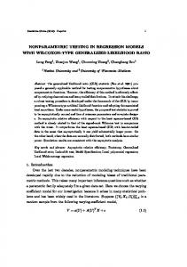
Lung Cancer Study
Survival Study of lung cancer in NI (Wilkinson, 1992). A total of 855 incident cases followed for 2 years. 50% dead by 6 months. Interested in who gets active treatment (and why)? Some 51.5% received no active treatment! Leads to a standard MLF analysis with Y=1 for treatment else Y=0. Some 5 covariates WHO, Age, Cell type, Metastases and Albumen. See example in next slide.
CASI, Templepatrick, N. Ireland, May 14-16th, 2014
14
Outline
Intro
LMs
Precision
MC
T-MC
Conc
Ref
App
CASI, Templepatrick, N. Ireland, May 14-16th, 2014
15
Outline
Intro
LMs
Precision
MC
T-MC
Conc
Ref
App
Conclusions
There is more see than suggested by Berk. Maximising the Precision minimizes the Multi-collinearity. Must be useful in sparse data situations with many categorical covariates. No loss of information on contrasts of interest For LMs and GLMs (and beyond) results are similar. Overall we have created some useful tools. We hope their use will improve practice.
CASI, Templepatrick, N. Ireland, May 14-16th, 2014
16
Outline
Intro
LMs
Precision
MC
T-MC
Conc
Ref
App
Acknowledgements The work in this paper was supported by two Science Foundation Ireland (SFI, www.sfi.ie) project grants. Professor MacKenzie was supported under the Mathematics Initiative, II, via the BIO-SI (www.ul.ie/bio-si) research programme in the Centre of Biostatistics, University of Limerick, Ireland: grant number 07/MI/012. Professor Peng is also supported via a Research Frontiers Programme award, grant number 05/RF/MAT 026.
CASI, Templepatrick, N. Ireland, May 14-16th, 2014
17
Outline
Intro
LMs
Precision
MC
T-MC
Conc
Ref
App
References A LTMAN, D. G. & R OYSTON, P. (2006). Statistics notes - The cost of dichotomising continuous variables. British Medical Journal, 332, 1080. B ELSLEY, D. A., K UH, E. & W ELSCH, R. E. (2004). Regression diagnostics: Identifying influential data and sources of collinearity. John Wiley & Sons, First edition. B ERK, R. (2008). Statistical learning from regression perspective. Springer, New York. C OHEN, J. (1988). Statistical power analysis for the behavioral sciences (2nd ed.). Hillsdale,NJ: Lawrence Erlbaum. C OX & S NELL (1989). Analysis of Binary Data. Chapman and Hall, Second edition. CRAN . R - PROJECT , (2009). R project. Retrieved 2010, from Package ’pwr’: http://cran.r-project.org/web/packages/pwr/pwr.pdf
E LWOOD, J. H., M AC K ENZIE, G. & C RAN, G. (1974). Observations on single births to women resident in Belfast 1962-66: Part I - Factors associated with perinatal mortality. J. Chron. Dis, 27, 517-535.
CASI, Templepatrick, N. Ireland, May 14-16th, 2014
18
Outline
Intro
LMs
Precision
MC
T-MC
Conc
Ref
App
References F ELDSTEIN, M. S., (1966). A binary variable multiple regression method of analysing factors affecting Peri-Natal mortality and other outcomes of pregnancy. Journal of the Royal Statistical Society. A 129, 61-73. F RØSLIE, K. F, R ØISLIEN, J., L AAKE, P., H ENRIKSEN, T., Q VIGSTAD, E. and V EIERØD, M. B.(2010). Categorisation of continuous exposure variables revisited. A response to the Hyperglycaemia and Adverse Pregnancy Outcome (HAPO) Study. BMC Medical Research Methodology, 10, 1471-2288. I SHAM, (1991). Statistical theory and modelling by edited by D.V. Hinkley, N. Reid, and E.J. Snell. Chapman and Hall. M AC K ENZIE, G. & P ENG, D. (2010). Properties of estimators in interval censored PH regression survival models. Submitted. Journal of the Royal Statistical Society. C. N IJENHUIS, A. & W ILF, H. S. (1978). Combinatorial Algorithms for Computers and Calculators. Academic Press, Second edition. P ENG , D. & M AC K ENZIE G. (2014). Discrepancy and choice of reference subclass in categorical regression models. In: Statistical Modelling in Biostatistics and Bioinformatics. Springer, Munich, 260 pages. CASI, Templepatrick, N. Ireland, May 14-16th, 2014
19
Outline
Intro
LMs
Precision
MC
T-MC
Conc
Ref
App
References P OCOCK, S. J., C OLLIER, T. J., DANDREO, K. J., D E S TAVOLA, B. L., G OLDMAN, M. B., K ALISH, L. A., L INDA, E. K. & VALERIE, A. M. (2004). Issues in the reporting of epidemiological studies: a survey of recent practice. British Medical Journal, 329, 883-887. R AO, C. R. & R AO, M. B. (1998). Matrix Algebra and its Applications to Statistics and Econometrics. World Scientific Publishing, Singapore, First edition. S HAPIRO, S. S. (1980). How to test normality and other distributional assumptions. statistical techniques, 3, 1-78. S MITH, O. K. (1961). Eigenvalues of a symmetric 3 × 3 matrix. Communications of the ACM. 4, 168. W ISSMANN, M., TOUTENBURG, H. & S HALABH, (2007). Role of Categorical Variables in Multicollinearity in Linear Regression Model. Technical Report. Department of Statistics University of Munich, Germany. Number 008. W ILLIAM, G. J. (2005). Regression III: Advanced methods. Lecture notes. Department of Political Science Michigan State University, America. http://polisci.msu.edu/jacoby/icpsr/regress3.
CASI, Templepatrick, N. Ireland, May 14-16th, 2014
20
Outline
Intro
LMs
Precision
MC
T-MC
Conc
Ref
App
Minimizing the Total Variance
Proof. Let nr = max(n1 , · · · , np ), and s ∈ {1, 2, · · · , p} (s 6= r ) be another choice of reference category, where nr > ns , then, from (17), the corresponding total variances are Vr = 1/nr + (1/nr + 1/ns ) +
p X
(1/nr + 1/nj )
j6=r ,s
and Vs = 1/ns + (1/ns + 1/nr ) +
p X
(1/ns + 1/nj ).
j6=r ,s
Since 1/nr < 1/ns , we have Vr < Vs , i.e., choosing nr = nmax minimizes the total variance.
CASI, Templepatrick, N. Ireland, May 14-16th, 2014
21
Outline
Intro
LMs
Precision
MC
T-MC
Conc
Ref
App
Canonical GLMs Canonical GLM for independent responses Yi with E(Yi ) = µi = g(θi ), θi =
k X
xui βu
u=0
is the linear predictor, βu = 0, . . . , k , represents the p regression parameters. Then the observed information matrix for β is Io (β) = (Oβ θT )(Oθ Oθ K )(Oβ θT )T = (Oβ µT )(Oθ Oθ K )−1 (Oβ µT )T .(11) When β0 is the intercept, we can re-express as the (p × p) matrix � P � P 0 w P i xci w0i Io (β0 , βc ) = (X 0 WX ) = P i i , (12) i xci xci wi i xci wi CASI, Templepatrick, N. Ireland, May 14-16th, 2014
22
Outline
Intro
LMs
Precision
MC
T-MC
Conc
Ref
App
Structural Weights
Table 2: Structural weights Distribution
Normal Exponential IG
Density(Mass) Function f (y ; µ, σ) = √ 1 f (y ; λ) = λe
2πσ −λy
−(y −µ)2 e 2σ2
1 f (y ; µ, λ) = ( λ 3 ) 2 e 2πy λy y!
−λ
Poisson
f (y ; λ) =
Binomial
f (y ; n, p) =
Geometric
f (y ; p) = (1 − p)y −1 p
Link function
wi
xβ = µ = θ
σ −2
−1
xβ = µ −λ(y −µ)2 2µ2 y
e � � n py (1 − p)n−y y
=θ
xβ = µ−2 = θ xβ = log(µ) = θ µ xβ = log( (1−µ )=θ µ xβ = log( (1−µ )=θ
(xi0 β)−2 λ (x 0 β)−3/2 4 i exp(xi0 β) exp(x 0 β) i (1+exp(x 0 β))2 i 1 1+exp(x 0 β) i
CASI, Templepatrick, N. Ireland, May 14-16th, 2014
23
Outline
Intro
LMs
Precision
MC
T-MC
Conc
Ref
App
Extension to Canonical GLMs For a single categorical variate across GLMs we can Show that the optimal choice depends on nr × ϕ(βˆ0 ). Show that we should choose the subclass where nr × ϕ(βˆ0 ) is max. Show that choosing nr = nmax is usually good. Show that when the observed allocation is uniform (n1 = n2 = · · · = np ) or near uniform the choice of reference subclass does not matter. Show there is an index to tell you when you need to worry about lack of uniformity. These results extend to GLMs with multiple categorical covariates. CASI, Templepatrick, N. Ireland, May 14-16th, 2014
24
Outline
Intro
LMs
Precision
MC
T-MC
Conc
Ref
App
Contrasts of Interest
Generally, such contrasts are conducted among the k regression coefficients. Then we have V (Z ) = C 0 V (βr )C V (Z ) = σ
2
k X
cj2 /nj
j=1
where c0 = 0 and c 0 1 = 0. Then Z does not depend on β0 and accordingly such contrasts are invariant to the choice of reference subclass.
CASI, Templepatrick, N. Ireland, May 14-16th, 2014
25
Outline
Intro
LMs
Precision
MC
T-MC
Conc
Ref
App
Generalization of V-C matrix The generalised Variance covariance matrix for GLMs is 1 −1 −1 1 I −1 (β0 , βc ) = nr ϕ(β0 ) .. . −1
−1 1 + (τ1 × 1 .. . 1
nr ) n1
−1 1 1 + (τ2 × .. . 1
nr ) n2
··· ··· ···
···
−1 1 1 .. . 1 + (τk ×
nr nk
, (13) )
where i[j] means subject i ∈ jth category, whence xji = 1 for i ∈ jth category, and τj = ϕ(β0 )/ϕ(β0 + βj ), nr and nj are the allocated numbers in the reference subclass and the jth subclass respectively, j = 1, 2, · · · , k . This matrix structure recurs in other settings (MacKenzie & Peng, 2013: Peng & MacKenzie, 2014).
CASI, Templepatrick, N. Ireland, May 14-16th, 2014
26