Classification and identification of recorded and synthesized impact sounds by practiced listeners, musicians, and nonmusicians Robert A. Lutfi, Eunmi Oh,a兲 Eileen Storm, and Joshua M. Alexander Department of Communicative Disorders and Waisman Center, University of Wisconsin, Madison, Wisconsin 53706
共Received 21 May 2004; revised 13 April 2004; accepted 25 April 2005兲 Three experiments were conducted to test the viability of a low-parameter modal model for synthesizing impact sounds to be used in commercial and psychoacoustic research. The model was constrained to have four physically based parameters dictating the amplitude, frequency, and decay of modes. The values of these parameters were selected by ear to roughly match the recordings of ten different resonant objects suspended by hand and struck with different mallets. In experiment 1, neither 35 professional musicians nor 187 college undergraduates could identify which of the two matched sounds was the real recording with better than chance accuracy, though significantly better than chance performance was obtained when modal parameters were selected without the previously imposed physical constraints. In experiment 2, the undergraduates identified the source corresponding to the recorded and synthesized sounds with the same level of accuracy and largely the same pattern of errors. Finally, experiment 3 showed highly practiced listeners to be largely insensitive to changes in the acoustic waveform resulting from an increase in the number of free parameters used in the modal model beyond 3. The results suggest that low-parameter, modal models might be exploited meaningfully in many commercial and research applications involving human perception of impact sounds. © 2005 Acoustical Society of America. 关DOI: 10.1121/1.1931867兴 PACS number共s兲: 43.66.Yw, 43.66.Fe 关AK兴
I. INTRODUCTION
Impact sounds, the sounds produced by objects coming in brief contact with one another, are abundant in nature and in music. They constitute an important class of sounds in the fields of physical and musical acoustics 共Morse and Ingard, 1968; Rossing and Fletcher, 1999兲, and they play a significant role in ongoing efforts to automate sound animation for computer gaming applications and interactive virtual environments 共Durlach and Mavor, 1995兲. This paper is concerned primarily with the use of impact sounds in psychoacoustic research, where they are the favored stimulus in studies of human sound source identification. The goal is to provide an initial evaluation of a low-parameter modal model for synthesizing impact sounds that could be practically applied in psychoacoustic studies of how listeners recover source attributes from sound. In most past psychoacoustic studies using impact sounds the sounds have been generated “live” or have been recorded from live sources 共cf. Carello et al., 1998; Freed, 1990; Kunkler-Peck and Turvey, 2000; Lakatos et al., 1997; Li et al., 1991; Repp, 1987; Warren and Verbrugge, 1984兲. Such manner of presentation ensures that most, if not all, acoustic information about the source is preserved in the sound reaching the listener’s ears, but there are drawbacks. Live sounds are difficult to control and replicate accurately without spe-
a兲
Present address: at Samsung AIT P.O. Box 111, Suwon, Korea 440-600; Electronic mail:
[email protected]
J. Acoust. Soc. Am. 118 共1兲, July 2005
Pages: 393–404
cial apparati. The time and cost of constructing such apparati can be great and is likely the reason that few studies have attempted to replicate the results of other laboratories using live sound. Sound recordings have an advantage in that they can be reliably replicated and easily manipulated. However, sound recordings are impractical in research applications where the acoustic cues must be precisely related to the physical dynamics of the sound-producing source 共Lutfi, 2001; Lutfi and Oh, 1994, 1997; Lutfi and Wang, 1999兲 or, as in gaming applications, where one requires real-time interactive or adaptive control over source parameters 共cf. Cook, 1996, 1997; Durlach and Mavor, 1995; Van den Doel, 1998; Van den Doel and Pai, 1996, 1998; Van den Doel et al., 2002兲. As a reaction to these problems there has been recent growing interest in physically informed 共PI兲 models for synthesizing impact sounds for use in both commercial and research applications 共Gaver, 1993a, b; Giordano and Petrini, 2003; Lakatos et al., 2000; Lutfi, 2001; Lutfi and Oh, 1997; Roussarie et al., 1998, and Takala and Hahn, 1992兲. This work uses what is known regarding the physics of vibrating bodies to exert greater control over relevant acoustic parameters and their relations. Gaver 共1993a兲 proposed an early working model of this type in which the vibrating object is represented as a bank of damped oscillators driven by an external force. Subsequent work has offered specific suggestions for how to select the parameters of this model based on the material and geometric properties of the object, the type of driving force, and the point at which the driving force is
0001-4966/2005/118共1兲/393/12/$22.50
© 2005 Acoustical Society of America
393
applied to the object 共Cook, 1996, 1997; Lambourg et al., 2001; Chaigne and Doutaut, 1997; Lutfi, 2001; Lutfi and Oh, 1994, 1997; Morrison and Adrien, 1993; Roussarie et al., 1998; Van den Doel, 1998; Van den Doel and Pai, 1996, 1998; Van den Doel et al., 2002兲. The product of these efforts in each case is a precise analytic representation of the stimulus that serves to specify the various sources of acoustic information for identification. The representation also affords the freedom in manipulating stimuli necessary to determine precisely how listeners make use of this information 共e.g., Lutfi, 2001; Lutfi and Oh, 1994, 1997兲. Though much work has already been undertaken using the physically informed approach, few studies have addressed the question as to how much detail is required in a PI model for it to be generally applicable in psychoacoustic research. Most published studies to date have been intended for applications in music and audio animation where the goal has been to reduce the computational load involved in the sound synthesis. These studies have mostly used similarity metrics to evaluate the degree to which listeners judge the synthesized sounds to “sound like” the real thing 共Charbonneau, 1981; Grey, 1977; Grey and Moorer, 1977; Van den Doel et al., 2002兲—a different criterion than would be required for many applications in psychoacoustic research. Where just-noticeable differences have been measured using forced-choice methods the primary concern has been with the perceptible effects of data reduction schemes applied to the acoustic waveforms 共Grey and Moorer, 1977; McAdams et al., 1999; Sandell and Martens, 1995兲. Such results bear only indirectly on the problem of determining the minimal number of parameters required of a PI model to produce an acceptable psychophysical approximation to live sound. The present study was undertaken to get some sense of the amount of detail required of a PI model for it to be of general use in psychophysical research. Our approach was to begin with a generic model having a small number of free parameters 共a large number of physical constraints兲 and to add complexity until certain criteria for psychophysical validity were met. For practical reasons, described later, we chose not to pursue the strictest criterion, which would be to require that real and synthesized sounds be indistinguishable from one another. Instead, the following three criteria were chosen: First, in forced-choice comparisons between realrecorded and synthesized sounds, highly trained listeners 共professional musicians兲 were required to identify the real sound with no greater than chance accuracy. Second, in a source identification task involving untrained listeners, realrecorded and synthesized sounds were required to produce no significant differences in performance or pattern of errors. Third, for a given number of free parameters satisfying the first two criteria, highly practiced listeners were required to be largely insensitive to the changes resulting from further increases in the number of parameters used to synthesize the sounds. As it turned out, the generic model with fewest parameters tested satisfied all three criteria. The results imply that in many cases low-parameter PI models can be applied with efficacy in psychoacoustic studies of human sound source identification using impact sounds. 394
J. Acoust. Soc. Am., Vol. 118, No. 1, July 2005
II. SOUND RECORDING AND SYNTHESIS
The general PI model that we have adopted is fundamentally the one proposed by Gaver 共1993a兲 and used in most current applications in psychophysical research referenced above. The sound-producing object is represented as a series of N coupled oscillators driven at some point xc by an impulse and damped by both external and internal frictional forces. The parameters of this model are a vector of N modal frequencies, n, with associated gain, Cn,x, and decay moduli, n that depend on the geometric and material properties of the source 共cf. Kinsler and Frey, 1962; Lutfi, 2001; Rossing and Fletcher, 1999兲. The gain values further depend on the location x where the radiated sound is measured and the point xc where the impulse is applied. The sound-pressure waveform radiated at x is given by N
y x共t兲 = 兺 Cn,x,xce−t/n sin共2nt兲.
共1兲
n=1
Allowing overall intensity to vary arbitrarily, the maximum number of free parameters of this model is 3N − 1. Our intent was to systematically vary the number of free parameters up to 3N − 1 to find the minimum number that would satisfy the three criteria for “psychophysical validity” previously stated. This turned out to be unnecessary as the model with fewest free parameters tested satisfied these criteria. We will refer to this as the physically least-informed 共PLI兲 model. The PLI model had four free parameters that were chosen to capture the gross acoustic effect of various physical properties of the object, how it was held, and how it was struck. Note that it is the physically informed constraints placed on parameter selection that distinguish the PLI model from a pure modal model in which parameters are selected without constraint to match those of the source signal. The first parameter specified the ratios n / 1 of the modal frequencies as is associated with the gross geometric dimensions of the object; i.e., its class or type. This parameter could take on one of two values depending on whether the object to be simulated was judged to have acoustic properties more like that of a bar or more like that of a plate. For the bar the frequency ratios were 1.00, 6.26, and 17.54; for the plate they were 1.00, 2.80, 5.15, 5.98, 9.75, 14.09, 14.91, 20.66, and 26.99. These values appear in standard acoustics texts as theoretical values representing ideal homogenous bars clamped at one end and loosely suspended circular plates 共e.g., Rossing and Fletcher, 1999兲. Higher frequency ratios given in these texts were not included as the frequencies would have been outside the audible range for the objects we selected for simulation. The second and third free parameters were the frequency, 1, and decay modulus,1, of the first partial. The frequency 1 was used to largely capture the effects of object size and material, while decay modulus 1 was used to approximate the degree of damping of the source resulting from internal friction and/or the manner in which the source was suspended by hand and struck 共Morse and Ingard, 1968兲. The decay modulus of the first partial further dictated the decay moduli of higher partials. For the bar these were constrained to vary in inverse proportion to the cube of frequency, n = 1共1 / n兲3 共cf. Morse and Ingard, 1968; Lutfi Lutfi et al.: Identification impact sounds
TABLE I. Description of objects used to produce sound recordings including hammers used and approximately where the objects were held and struck. Point of contact
Object
Description
Hammer
A
Small pipe, holes each end, ⬃6 ⫻ 1 in.2 Small ceramic plate, ⬃6-in. diameter Square hollow aluminum tube ⬃3 ft⫻ 1.5 in. Rectangular wood slab, cedar, ⬃18⫻ 0.5⫻ 6 in.3 Small juice glass
All plastic, handle end metal head- pointy end Plumb permabond plastic end metal head- pointy end metal head- pointy end Plumb permabond plastic end metal head- pointy end metal head- pointy end
1 4
way down
1 4
way down
1 4
way down
1 4
way down
metal head- pointy end All plastic, handle end
1 4 1 4
B C D E F G H
I J
Large hollow iron pipe, rusted ⬃1.5 ft⫻ 4 in. Small ceramic bowl, ⬃5-in. diameter Light metal rectangular strip with sides folded over, ⬃12⫻ 1 in.2 Small hollow metal chime, ⬃5 ⫻ 0.3 in.2 1 Thin brass rod ⬃3 ft⫻ 8 in.
and Oh, 1997; Lutfi, 2001兲. For the plate they varied in inverse proportion to frequency 共Rossing and Fletcher, 1999兲. The fourth and final parameter was spectral tilt, linear in dB/oct, which specified the relative gain values Cn,x / C1,x of the partials. The values of spectral tilt could be either positive or negative and were used to roughly approximate the effects of the point of impact, type of hammer used, and the manner in which the source was held. For example, a soft mallet produces an impulse that increases more gradually over time, resulting in a loss of high frequencies in the driving force and concomitant attenuation of higher frequency partials in the response 共Fletcher and Rossing, 1991, pp. 547–548兲. Altogether ten stimuli were synthesized using the PLI model. The parameters of the model in each case were selected by ear by a laboratory assistant so as to roughly match the sound recordings of ten everyday resonant objects suspended by hand and struck with different hammers. Details of the stimulus generation for the matching phase of the study were the same as those used in the experiments as described in Sec. III A. After one or more comparisons the assistant would adjust one or more of the free parameters of the modal model in an attempt to reconstruct a synthesized sound that was a closer match to the recording. There was no systemic procedure or order for selecting parameters; rather the selection was made simply by trial and error. Again, the intent was not to make sounds indiscriminable from one another, only to achieve a realistic qualitative match. A description of the objects used in these experiments is given in Table I along with a description of the hammers used, and an indication of approximately where the objects were held and struck. These objects were selected because they made a variety of different sounds and because they could be readily found in our lab and machine shop. There J. Acoust. Soc. Am., Vol. 118, No. 1, July 2005
Grip
bottom 3 4
middle 3 4
bottom
way down middle
3 4
way down
3 4
way down
3 4
way down
way down
3 4
way down
way down
3 4
way down
top 1 4
way down
way down top
were no other special criteria for selecting these objects. We chose the objects to be held by hand because we were interested in the sounds that occur naturally when a person picks up an object and strikes it to determine its physical properties from sound. Table II gives the values of the model parameters chosen for each of the ten objects used in the study. Recordings were made in a sound-treated room using a Shure SM81 directional microphone 共all-pass setting兲 and a USBpre 16-bit analog-to-digital conversion system that sampled at a 44.1-kHz rate. The microphone was suspended on a boom and was pointed directly toward the sound source at approximately 2 / 3 m from the sound source. Both synthesized sounds and sound recordings were edited to be 1 s in duration from the beginning of the impact by applying a 10 -ms cosine-squared ramp at offset. In all but a few cases the sounds decayed to inaudibility within 1 s.
TABLE II. Parameter values of the modal model used in experiments I–III. See Table I for description of simulated objects and see text for description of acoustic parameters. Object
n / 1
1 共Hz兲
1 共s兲
Cn / C1 共dB/oct兲
A B C D E F G H I J
Plate Plate Plate Plate Plate Plate Plate Plate Bar Bar
5862 1532 407 808 1827 1591 1789 1460 2109 3521
0.103 0.065 0.872 0.037 0.194 0.397 0.177 0.069 0.163 0.179
−6 0 −6 −6 −60 0 1 0 −12 −6
Lutfi et al.: Identification impact sounds
395
III. EXPERIMENT 1. CLASSIFICATION OF IMPACT SOUNDS AS REAL OR SYNTHESIZED
The first experiment of the series addressed the first criterion for psychophysical validity. The ten real-recorded sounds were paired with their synthesized counterparts to create a sequence of ten, two-interval, forced-choice identification trials. Thirty-four members of the Madison Symphony Orchestra 共MS listeners兲 and 187 undergraduate students from the University of Wisconsin—Madison 共UW listeners兲 were asked to identify on each trial which of the two sounds corresponded to the real-recorded sound. We wished to determine whether either group would be able to identify the real-recorded sound with greater than chance accuracy. Note that the classification task differs from the task in which a listener is asked to give a subjective judgment regarding the perceived “realism” of a sound. The former has correct response, whereas the latter does not. As a control a different group of UW listeners was asked to identify the real-recorded sounds when paired with synthesized sounds for which the frequencies and decay moduli were selected at random over roughly the same range of values used in the first experiment. A. Procedure
The details of the procedure were slightly different for the MS and UW listeners. For the UW listeners the sounds were played in a large 16.8-m-wide by 17.5-m-long, twostory high, octagon-shaped, lecture hall over a modern, builtin, four-speaker, PA system 共TOA Model F-605W兲. The frequency response of the speakers was flat 共±5 dB兲 from 0.1 to 15.0 kHz. The walls of the lecture were largely covered by curtains offering little in the way of hard-reflecting surfaces. Listeners sat at different points in the room but were never less than 3 m away from the closet wall and never less than 4 m away from the closest speaker. For the MS listeners the sounds were played on the stage of a large orchestra concert hall 共where the MS listeners were seated兲 over a pair of small Acoustic Research speakers with built-in amplifiers. Curtains surrounded the back of the stage and the listeners closest to the speakers were seated about 4 m away. The frequency response of the speakers was flat 共±5 dB兲 from 0.2 to 15.0 kHz. For both groups of listeners the sounds were played at the 44.1-kHz rate with 16-bit resolution using a DELL notebook with an on-board Sound-Blaster Card. Sound level was adjusted to be at a comfortable listening level 共roughly 65– 70 dB SPL兲 near the center of each listening environment. The two sounds played on each trial were separated by 0.5 s with trials separated by approximately 8 s. Listeners were instructed that on each trial they would hear a pair of sounds corresponding to a common everyday object struck by a mallet. They were told that one of the sounds was a recording of the real object while the other was created artificially on a computer using mathematical equations—their task was to indicate which of the two sounds corresponded to the recording of the real object. Listeners marked their answers in pencil on a standard bubble sheet for later scoring by the UW grading center. No feedback was given on each trial as to which response was cor396
J. Acoust. Soc. Am., Vol. 118, No. 1, July 2005
FIG. 1. The percentage of UW listeners that obtained each of the possible percent correct scores in the real versus synthesized classification task 共experiment 1兲 is shown along with the predicted percentages given that true performance for all listeners was chance 共dashed line兲. Where asterisks are shown the obtained percentages are significantly greater than would be predicted assuming that true performance for all listeners was at chance.
rect. UW listeners were also asked to rate their own musical ability on a 5-point scale from “can’t carry a tune” to “highly-trained professional musician.” For their participation the UW listeners received extra credit for a class in communicative disorders; the MS listeners received candy. The ten trials can be heard at http://www.aip.org/pubservs/ epaps.html, the correct responses are respectively, 1st, 1st, 2nd, 1st, 2nd, 2nd, 2nd, 1st, 1st, 1st. B. Results and discussion
Figure 1 shows the proportion of UW listeners that obtained each of the possible percent correct scores. The dashed line represents the predicted proportions, based on binomial probabilities, given that true performance was at chance; asterisks denote the obtained proportions that are significantly greater than would be predicted assuming true performance was at chance 共N = 187, p ⬍ 0.01兲. Overall, the mean score of the UW listeners was 55.2% correct, not much better than chance. However, Fig. 1 shows that the mean score is not exactly representative of the “typical” listener since a disproportionate number of listeners scored both well above and well below chance. The results suggest that many listeners were able to identify some general quality that distinguished the two classes of sounds, but that they were about equally likely to identify this quality with the real as with the synthesized sounds. The pattern of results was much the same for the MS listeners, as is shown in Fig. 2. The mean score for MS listeners was 49.1% correct, slightly less than the UW listeners, with a larger proportion of MS listeners scoring well below chance. A correlational analysis of the musical ability ratings of the UW listeners also failed to indicate a relation between musical ability and performance. Interestingly, the mean performance of UW listeners who rated themselves as “highly-trained musicians” 共N = 30兲 was, like the MS listenLutfi et al.: Identification impact sounds
FIG. 2. Same as Fig. 1 except percentages are for MS listeners.
ers, below chance. The failure to obtain an effect of musical training is, perhaps, not surprising given that past studies have obtained mixed results regarding the effect of musical training. Spiegel and Watson 共1984兲 report that musicians generally perform better on frequency discrimination tasks than nonmusicians. Burns and Houtsma 共1999兲 report that musicians are better at detecting harmonicity. Closer to the present study, however, Eagleson and Eagleson 共1947兲 report that musicians are not much better at identifying musical instruments from isolated notes than college students and that neither group is very good. We might speculate as to the reason for the extreme scores above and below chance. The difference was subtle, but, to our ears the synthesized sounds had what might be described as a “pure” or “musical” quality that distinguished them from the real-recorded sounds. Acoustically, we suspect this was due to the broader bandwidth of the partials in the real-recorded sounds, the presence of additional modes, and the interaction 共“beating”兲 among modes. The synthesized sounds also differed in having uniform attack properties; note that no attempt was made to model the interaction between the hammer and the vibrating object in this synthesis. Figure 3 gives a breakdown of percent correct performance for each item 共symbol number兲 for each group of listeners. The figure shows clear differences in performance across items with good agreement between groups. It also shows that a few items in each case were responsible for the extreme scores: the large rusty pipe, ceramic bowl, and metal strip yielding scores below chance; the chime, wood slab, and juice glass yielding scores above chance 共N = 2210, p ⬍ 0.001兲. We had hoped that such differences would provide further insights into the reason for the extreme scores; however, the particular grouping of items offers no obvious clues. Lakatos et al. 共1997兲 report a similar result in which listeners more often than chance misidentified the shape of struck bars from their impact sounds. Though their study involved a very different type of judgment it is in keeping with the present results in showing consistent confusions for certain items. J. Acoust. Soc. Am., Vol. 118, No. 1, July 2005
FIG. 3. Comparison of percent correct performance for UW and MS listeners in the real versus synthesized classification task 共experiment 1兲 broken down by stimulus item. Letter symbols denote the different stimulus items as listed in Table I. Diagonal represents equal scores for the two groups.
Finally, to ensure that chance performance did not result from a simple failure of listeners to understand the task or to perform their best, we ran a control experiment. A second group of 158 UW listeners was given an easier task in which the synthesized sounds were created by selecting a random number of tones 共from one to nine兲 with random frequencies uniformly distributed between 100 and 10000 Hz, and random decay moduli uniformly distributed from 0 to 0.8 s. All other aspects of the experiment were the same as before. The results are shown in Fig. 4. Mean performance in this case was 81.5% correct, well above chance 共N = 1580; p ⬍ 0.001兲.
FIG. 4. Same as Fig. 1 except percentages are for a separate group of UW listeners who participated in a control experiment in which the synthesized sounds were created by selecting a random number of tones with random frequencies and decay moduli 共see text for further details兲. Lutfi et al.: Identification impact sounds
397
for psychophysical validity. The goal was to determine whether there would be any significant differences in source identification performance for the real-recorded and synthesized sounds. A. Procedure
FIG. 5. Visual display used in experiment 2 for sound source identification.
The results fail to support a significant contribution of motivational or other extraneous factors to the chance performance obtained in the first experiment. IV. EXPERIMENT 2. SOURCE IDENTIFICATION BASED ON REAL AND SYNTHETIC IMPACT SOUNDS
Despite the apparent ability of some listeners to detect a difference in quality between the real-recorded and synthesized sounds, the general failure of both UW and MS listeners to reliably identify the real-recorded sound satisfies our first criterion for psychophysical validity. This result does not, however, preclude the possibility that overall performance and/or the pattern of errors would be very different for the two types of sounds if listeners were asked to identify the sound source. It is entirely possible, for example, that the synthesized version of the juice glass sounded nothing like a juice glass to our listeners, even though it sounded quite real. One obvious way to test this possibility would be to obtain perceived similarity ratings from listeners. The problem with this approach is that it tells us little about the effect of the synthesis on identification—our primary goal. Different juice glasses, afterall, make different sounds. Hence, synthesized and real versions may be perceived as dissimilar but both may still equally likely be identified as a juice glass. The next experiment was undertaken to test the second criterion
Five matched stimulus pairs were selected for this experiment from the ten used in experiment 1. We used only a subset of all pairs as we did not wish to tax the demands of memory and attention by providing too large a number of response alternatives. The particular sources selected were items A–E 共see Table I兲. These sources were selected because their gross material and geometric properties were largely evident from photographed images and because they were easy to describe to listeners. Figure 5 shows these images exactly as they were seen by listeners throughout the experimental trials. A brief description of each object and the hammer used 共per Table I兲 was given to listeners prior to experimental trials. The ten stimuli corresponding to the five matched pairs were used to construct ten single-interval, five-alternative, identification trials. One of the stimuli 共either real-recorded or synthesized兲 was selected at random without replacement and played on each trial. Listeners were instructed on each trial to “pick the picture that best matches the sound.” As in experiment I, listeners marked their answers in pencil on a standard bubble sheet for later scoring by the UW grading center; no feedback was given on each trial. The experiment was conducted approximately one month after experiment 1 on the same class of UW undergraduates 共190 listeners altogether, mostly the same as those participating in experiment 1兲. All other aspects of the experiment were identical to experiment 1. B. Results and discussion
Figure 6 shows the confusion matrices resulting from separate analyses of the responses to the real-recorded and synthesized impact sounds 共left and middle panels, respectively兲. The relative proportion of responses is indicated by number and by grayscale with darker regions representing fewer responses. Correct responses are represented by cells that fall on the positive diagonal. The figure makes clear at a
FIG. 6. Confusion matrices from source-identification experiment 共experiment 2兲. The relative proportion of responses is indicated in grayscale with darker regions representing fewer responses. Entries are the actual proportions of responses. Responses of the first group of UW listeners to the real-recorded and synthesized impact sounds are analyzed separately in the left and right panels, respectively. Responses of the second group of listeners to the real-recorded sounds at the same positions in the sequence as the synthetic sounds are shown in the right panel 共see text for further details兲. 398
J. Acoust. Soc. Am., Vol. 118, No. 1, July 2005
Lutfi et al.: Identification impact sounds
FIG. 7. Left panel: The probability of each response associated with each item 共grayscale values in the first two panels of Fig. 6兲 is given for both the real-recorded and synthesized sounds from the first group of listeners. Error bars represent 95% confidence intervals. Middle panel: Shows agreement in responses to the first and second presentations of the real-recorded sounds for the second group of listeners. Right panel: Shows agreement in responses to the real-recorded sounds of the second group of listeners and the synthesized sounds for the first group of listeners, where the synthesized sounds occurred in the same positions in the trial sequence 共see text for details兲.
glance the degree of agreement between the two confusion matrices. In both cases, for example, the item most often correctly identified is the rectangular wood slab 共item D兲. And, with the exception of the synthesized ceramic plate 共item B兲, the items least often identified correctly are the small pipe 共item A兲 and the small juice glass 共item E兲 in both cases. There are also some differences in the confusion matrices. For example, the synthetic sound corresponding to the small pipe 共item A兲 is often identified as belonging to the square hollow rod 共item C兲, but for the real-recorded version this is rarely true. The left panel of Fig. 7 better shows the extent of the differences. Plotted is the probability of each response associated with each item for both the real-recorded and synthesized sounds 共i.e., the values indicated by grayscale in Fig. 6兲. Error bars give the 95% confidence intervals for each value assuming binomial error 共N = 190兲. Perfect agreement between the two confusion matrices would result in all points falling on the positive diagonal. It is clear from the figure that many values deviate significantly from the diagonal. There are at least two factors, other than perceived differences between the real-recorded and synthesized sounds, which could contribute to the discrepancies between these confusion matrices. The first is internal inconsistencies in judgments—the tendency of listeners to make a different judgment in response to a repeated presentation of the same stimulus. The second is order effects—the influence that prior judgments can have on subsequent judgments. A control experiment was conducted to evaluate the relative contributions of these factors. The identification experiment was repeated on a new group of UW undergraduates 共N = 150兲 with the synthesized sounds simply replaced by their realrecorded counterparts at their same positions in the sequence of trials. Listeners in this experiment, thus, had two “looks” at the real-recorded sounds. The middle panel of Fig. 7 shows the agreement in the responses for the first and second “looks,” denoted real1 and real2, respectively. The deviations from the diagonal in this case reflect the combined contribution of internal inconsistencies and order effects; they are on the same order of magJ. Acoust. Soc. Am., Vol. 118, No. 1, July 2005
nitude as those of the left panel of Fig. 7, which shows the agreement in responses for the real and synthesized sounds obtained from the first group of listeners 共data shown in the first two panels of Fig. 6兲. The good agreement suggests that internal inconsistencies and/or order effects, not perceived differences between real and synthesized sounds, are responsible for the discrepancies in responses. The right panel shows the agreement in responses for the real-recorded sounds of this experiment and the synthesized sounds from the first group of listeners. This comparison controls for order effects inasmuch as the two sets of sounds occurred in the same positions in the trial sequence. Here, the agreement in responses is quite good, indicating that much of the variability in judgments was due to order effects and not perceived differences between the real and synthesized sounds. Reinforcing this conclusion is the confusion matrix for the real-recorded sounds of this experiment, given in the right panel of Fig. 6. Here too the agreement between responses is quite good. Overall these results demonstrate excellent agreement between the identification responses given to the real-recorded and synthesized sounds once the effects of order in the sequence are partialled out. V. EXPERIMENT 3. COMPARISON OF HEADPHONE AND SPEAKER PRESENTATION
To obtain reliable estimates of the distributional properties of listener responses in experiments 1 and 2 it was necessary to recruit a large number of participants. The most practical way of doing this was to present stimuli once and at the same time to a large group of listeners over speakers. This approach, of course, is problematic in that the acoustics of any setting in which sounds are delivered over speakers can potentially have an adverse effect on the quality of the sound reaching the listener’s ear. Moreover, in many research applications in psychoacoustics involving the identification of sound sources, the sounds are likely to be delivered over headphones, not over speakers. Two observations suggest that room acoustics was not a significant factor contributing to the results of experiments 1 and 2: the good performance Lutfi et al.: Identification impact sounds
399
FIG. 8. Percent correct performance in the real-recorded versus synthesized classification task for UW listeners, headphone versus speaker presentation, broken down for each stimulus item. Letter symbols denote the different stimulus items as listed in Table I. Mu gives mean performance across items. Diagonal represents equal scores for the two listener groups.
of UW listeners in the control experiment to experiment 1, and the fact that sounds were delivered to MS listeners in a concert hall designed to reduce reverberation. To be confident, however, that room acoustics was not a factor we replicated experiments 1 and 2 using a smaller group of listeners with sounds delivered over headphones. A. Procedure
All details regarding stimulus generation and procedure were identical to those of experiments 1 and 2 except that the sounds were presented diotically over circumaural headphones 共Beyerdynamic DT990兲 to individual listeners seated in a sound-isolated room. Also, for experiment 2 the visual display 共Fig. 5兲 was viewed on a computer monitor rather than on a large projection screen. A total of 40 UW undergraduates were recruited for these experiments. None had participated in the previous experiments. We did not want previous exposure to the stimulus items to confound the comparison between headphone and speaker presentation. As before the students received extra credit in an introductory class in communication disorders for their participation. B. Results and discussion
Figure 8 compares percent correct performance using speaker and headphone presentation in the real-recorded versus synthesized classification task which tested our first criterion for psychophysical validity. The data for speaker presentation are taken from the 187 UW listeners of experiment 1. Performance is broken down by stimulus item with letter symbols denoting each item as listed in Table I. The diagonal represents equal scores for the two presentation modes. We expect some variability about the diagonal given the differences in the two groups of listeners used for the two presen400
J. Acoust. Soc. Am., Vol. 118, No. 1, July 2005
FIG. 9. Same as Fig. 8 except for the source identification task. Upper-case letters indicate real-recorded items, lower-case letters indicate synthesized counterparts.
tation modes. Importantly, however, there is no evidence of an advantage of headphone presentation. Indeed, average performance for headphone presentation 共indicated by the Greek letter mu兲 is slightly worse 共48.3% correct兲 than average performance for speaker presentation 共55.2% correct兲. A similar outcome is obtained for the headphone replication of the source-identification experiment 共experiment 2兲. Figure 9 gives performance broken down by stimulus item in the same manner as Fig. 8. The upper-case letters denote the real-recorded items while the lower-case letters denote their synthesized counterparts. The figure shows generally good agreement between the headphone and speaker presentation modes with headphone presentation, once again yielding slightly worse performance overall 共47.5% correct兲 than speaker presentation 共58.2% correct兲. We conclude based on these results that room acoustics had little to do with the poor performance of listeners in experiments 1 and 2. VI. EXPERIMENT 4. DISTINGUISHING SYNTHESIZED IMPACT SOUNDS WITH DIFFERENT NUMBERS OF FREE PARAMETERS
The results of experiments 1–3 suggest that the PLI model might justifiably be applied to source identification tasks in which the response categories are rather broad; e.g., wood slab vs. metal pipe vs. ceramic plate, etc. What, however, of more subtle distinctions within these categories? Consider, for example, the task of distinguishing from sound a metal bar that is bent from one that is true. Here, differences in the frequency ratio and/or relative decay moduli of modes are likely to be potential cues. But, because the PLI model constrains these to be constant, it would not be applicable in this case. Recognizing that no single model is likely to be suitable for all identification tasks, we would like to have some measure of the perceptual consequences associated with particular model constraints. The approach we take Lutfi et al.: Identification impact sounds
in the next experiment is to measure the listener’s ability to detect changes in the acoustic waveform that result when these constraints are relaxed; that is, when a greater number of free parameters are allowed. We argue that a PI model should have a broader potential for application to the extent that highly practiced listeners are insensitive to such changes. A. Procedure
Unlike the previous experiments, our goal here is simply to determine whether listeners can detect the acoustic effect of relaxing constraints of the PLI model. We chose, therefore, to simulate a single sound source so that listeners would not potentially confuse a change in source with a change in model constraints. Two sets of sounds, 100 samples each set, were constructed according to the PLI model as described in Sec. II. For both sets the nominal values of parameters were chosen to simulate the sound of a common tuning fork 共a homogeneous bar clamped at one end and struck at the other兲: 1 = 461 Hz, 1 = 0.55 s, and Cn / C1 = 6 dB/ oct. This source had been used in the previously referenced studies by Lutfi 共2001兲 and Lutfi and Oh 共1994, 1997兲 共real-recorded and synthesized versions can be heard at http://www.aip.org/ pubservs/epaps.html兲. Different samples within each set of 100 sounds were obtained by jittering the frequencies of the partials at random about their nominal values. The jitter was a multiplier of these values and was normally distributed with mean 1.0 and standard deviation in different conditions of 0.1, 0.2, and 0.3. The nominal values of the decay moduli varied accordingly, in inverse proportion to the cube of frequency. For the first set of sounds the frequencies of partials covaried; the value selected for 1 dictated the values of 2 and 3 according to the ideal ratios given in Sec. II. In effect, these sounds had one free parameter. For the second set of sounds the frequencies of the three partials varied independently, thus relaxing one of the constraints of the PLI model. These sounds, in effect, had three free parameters 共one for each partial兲. A second condition was also run in which both the frequencies and the decay moduli of partials in the second set varied independently 共six free parameters兲; although, once again the values of frequency and decay were identically distributed. On each trial one sample from both sets was drawn at random and played over headphones 共Sennheiser HD520兲 to the right ear of listeners seated in a double-wall, IAC sound-attenuation booth. All sounds were generated at a 40-kHz rate using a Tucker-Davis 16-bit D/A conversion system with 20-kHz low-pass antialias filter. In the standard two-interval, forced-choice procedure, the listener’s task was to choose the sound drawn from the one-free-parameter set 共most constrained model兲. In physical terms the task was principally like that of identifying which of two metal bars is true, as in the example described above. For an ideal homogenous bar 共without bend兲 the frequency ratios of modes are given by the one-free-parameter set; these are the ideal ratios given for the struck clamped bar. For a bent bar the frequency 共and decay兲 ratios would deviate from ideal as for the three- and six-free parameter sets. Also, note that because the frequencies and decay moduli of the J. Acoust. Soc. Am., Vol. 118, No. 1, July 2005
FIG. 10. Percent correct performance of the five listeners 共panels兲 in both conditions 共different symbols兲 of experiment III is plotted as a function of the standard deviation of the frequency jitter of partials 共see text for details兲. Circular symbols denote the condition for which frequency alone was jittered and squares denote the condition for which both frequency and decay was jittered independently. Each symbol with error bar represents the mean and standard error of five estimates obtained on different days, 100 trials each estimate.
partials were identically distributed for the two sets of sounds the listener could not perform above chance by basing decisions on simple differences in frequency or decay. Listeners were given feedback after each trial and they were instructed to use the feedback during training to identify the quality difference between the two types of sounds. Five UW-Madison students ranging in age from 20 to 26 years were paid at an hourly rate for their participation in the experiment. They were highly practiced in the task, each receiving 1000 or more trials of training before data collection began. B. Results and discussion
Figure 10 shows the percent correct performance of the five listeners 共panels兲 in both conditions 共different symbols兲 as a function of the standard deviation of the frequency jitter. As the standard deviation of the jitter is increased we expect performance to improve since the frequency ratios of the three- and six-free parameter set will deviate more from the ideal values of the one-free parameter set. Circular symbols give the data for the three-free parameter set in which frequency alone was jittered; squares give the data for the sixfree parameter set in which both frequency and decay were jittered independently. Each symbol with error bar represents the mean and standard error of five estimates obtained on different days, 100 trials each estimate. The mean and stanLutfi et al.: Identification impact sounds
401
dard error of the estimates across listeners is given in the lower right panel. The pattern of results is quite similar for the five listeners and for the two conditions. Percent correct performance improves from near chance for 10% standard deviation in jitter to near 70% correct for 30% standard deviation in jitter. The results of this experiment show that highly practiced listeners are, indeed, capable of discriminating the difference between sounds synthesized with different numbers of free parameters. However, for the difference to be reliably detected the amount of jitter in the free parameters must be exceedingly large, 30% or greater. Note by comparison that the difference limen for a change in decay, for durations greater than 10 ms, is less than 20% 共Jarvelainen and Tolonen, 2001; Schlauch et al., 2001兲; the difference limen for a change in frequency it is but a fraction of a percent 共Wier et al., 1977兲. Increasing the number of free parameters from three to six did little to improve performance. This is noteworthy because six parameters is the largest number of parameters that may freely vary in this case while holding the relative levels of partials constant. While it is possible that sounds with a greater number of partials 共hence, a greater possible number of free parameters兲 might have yielded a different result, the failure to obtain even a small improvement in performance indicates that listeners are rather insensitive to the acoustic effect of increasing the number of free parameters beyond three. The present experiment was conducted using a single simulated source under a restricted set of conditions, so it is by no means clear that the same result would be obtained when simulating other sources under other conditions. Still, the principle design of the experiment is such that it provides, at least, a basis for estimating the minimum number of free parameters that are likely to be needed for a given application. For the tuning fork simulated here, there is a diminishing return of including more than the first three free parameters inasmuch as the effect on the acoustic waveform of including additional free parameters goes largely unnoticed by trained listeners given feedback in the two-interval, forced-choice task. In this one case, at least, the results are in keeping with those of experiments 1–3, and largely satisfy our third criterion for psychophysical validity. VII. GENERAL DISCUSSION
Understanding how we use sound to identify objects and events in the world is one of the most significant challenges for contemporary research on hearing 共cf. Bregman, 1990; Gibson, 1966兲. Yet, because of the multifarious nature of the stimulus progress has been limited. Ideally, one would like to have a precise representation of the stimulus that would allow predictions for performance and the types of errors expected based on the different available cues for identification and the manner in which they covary. Such a representation is difficult to achieve in the case of real or recorded sounds. It can be achieved through the analytic expressions of PI models, but only to the extent that these models faithfully represent the acoustic properties of the resonant sources they simulate. 402
J. Acoust. Soc. Am., Vol. 118, No. 1, July 2005
The present study was undertaken to provide some measure of the detail required of a PI model for it to have meaningful application in studies of human sound source identification from impact sounds. Since each application places different demands on a model, one can only go so far in generalizing beyond the present results. We have investigated but a few exemplars of a class of resonant objects that is indeterminately large; hence, there are likely to be many types of classifications for which these results do not apply. 共A notable example pertains to the manner of impact, since little effort was made to model this feature of the sound event.兲 Neither do these experiments permit us to determine the basis for classification—the wood slab, for example, could have easily been classified based on its material properties alone from the decay of a single partial 共cf. Lutfi and Oh, 1994, 1997; Wildes and Richards, 1988兲. Notwithstanding these qualifications, the results do, at least, suggest that a modal model with as few as three to four free parameters may be adequate for many applications in psychoacoustic research involving impact sounds produced by relatively simple resonant sources. This model produced sounds that professional musicians and college undergraduates alike could not recognize as synthesized versus real with better than chance accuracy. And, it produced sounds that yielded the same level of identification accuracy and largely the same pattern of errors when listeners where asked to identify the source. While these are not the only or even the strictest criteria for psychophysical validity, they are two meaningful criteria that go some way in encouraging a physically informed approach. Other studies have used different criteria for evaluating psychophysical validity, but with an eye towards achieving different goals. Grey and Moorer 共1977兲 and McAdams et al. 共1999兲, for example, adopted a strict criterion by challenging highly trained musicians to detect any difference between real-recorded and synthesized sounds. These studies were undertaken with the goal of reducing the computational load required to produce a transparent synthesis of notes played by musical instruments. The various algorithms used to reduce data 共e.g., smoothing of the spectral and temporal envelope, forced harmonicity, and the like兲 did not and were not intended to have a specific representation in the parameters of a PI model. Also, because the goal was to synthesize a very specific and small set of musical instrument sounds, a strict “no-differences-detected” approach was both meaningful and feasible. The same cannot be said for the present study where a small number of resonant objects are sampled to model an indefinitely large class of naturally occurring impact sounds. Similar differences in goals are noted in the studies of Charbonneau 共1981兲, Sandell and Martens 共1995兲, and Grey 共1977兲 where somewhat different techniques were used to synthesize musical instrument tones. A study whose goal was much closer to that of the present study was conducted by Van den Doel et al. 共2002兲. These authors had listeners rate the perceived dissimilarity between recorded and synthesized versions of the impact sounds produced by a ceramic bowl and metal vase. A 10 point scale was used with a rating of 1 corresponding to “no perceived difference.” The synthesized sounds were conLutfi et al.: Identification impact sounds
structed according to the modal model given by Eq. 共1兲; a phase-unwrapping algorithm was used to estimate the modal parameters from the recordings. The independent variable of interest was the number of audible 共unmasked兲 modes used in the synthesis. Perceived dissimilarity generally decreased as the number of modes increased, however there was a precipitous drop to “no perceived difference” at about six modes. While it is not possible to draw direct comparisons to the present study, the results nonetheless suggest that a realistic synthesis for simple resonant sources, like those used in the present study, can be achieved with relatively few modal parameters. This is consistent with our finding that highly practiced listeners are largely insensitive to an increase in free parameters such that would be required to model more specific differences between these sound sources 共experiment 4兲. The question of specificity is a larger problem that clearly requires further study. Several authors have offered analytic treatments of the acoustic relations that would uniquely identify specific source attributes, such as size, shape, and material, despite variation in other attributes 共Jenison, 1997; Kunkler-Peck and Turvey, 2000; Lutfi, 2001; Wildes and Richards, 1988兲. Few studies, however, have tested whether listeners are, in fact, sensitive to such relations. Two studies by Lutfi 共2000, 2001兲 are particularly relevant in this regard. In both, simulations were conducted in which the effect of sensory noise was estimated by introducing small perturbations in the acoustic parameters of the modal model. The magnitude of the perturbations for each parameter was estimated to be consistent with psychoacoustic data describing listener sensitivity to differences in the frequency, amplitude, and decay of single tones 共cf. Jesteadt et al., 1977; Schlauch et al., 2001; Wier et al., 1977兲. The results show that quite small perturbations, as would be associated with sensory noise, can significantly obscure relevant acoustic relations, even when variation in the acoustic signal is largely dominated by physical variation in the source. The results suggest that the acoustic relations relevant to particular identification tasks may, to a much greater extent than previously anticipated, be vulnerable to information loss in the auditory system. Such a conclusion would go some way in explaining the present failure to find significant differences in the listeners’ response to real-recorded and synthesized impact sounds. Though the results of this study do not bring us much closer to understanding how listeners identify simple sound sources, they do at least support the use of simple PI models as a means of approaching the problem.
ACKNOWLEDGMENTS
This research was supported by a grant from the NIDCD 共R01 CD01262-10兲. The authors wish to thank Robert Kim Todd and Gregory Minx for their technical support, Michi Adelmund and Karen Malott for assistance in data collection, and Dr. Armin Kohlrausch, Dr. Douglas Keefe, and three anonymous reviewers for helpful comments on an earlier version of this manuscript. J. Acoust. Soc. Am., Vol. 118, No. 1, July 2005
Bregman, A. S. 共1990兲. “Auditory Scene Analysis” 共M.I.T. Press, Cambridge, Massachusetts兲. Burns, E. M. and Houtsma, A. J. M. 共1999兲. “The influence of musical training on the perception of sequentially presented mistuned harmonics,” J. Acoust. Soc. Am. 106, 3564–3570. Carello, C., Anderson, K. A., and Kunkler-Peck, A. J. 共1998兲. “Perception of object length by sound,” Psychol. Sci. 9, 211–214. Chaigne, A., and Doutaut, V. 共1997兲. “Numerical simulations of xylophones. I. Time-domain modeling of the vibrating bars,” J. Acoust. Soc. Am. 101, 539–557. Charbonneau, G. R. 共1981兲. “Timbre and the perceptual effects of three types of data reduction,” Comput. Music J. 5共2, 10–19. Cook, P. R. 共1996兲. “Physically informed sonic modeling 共PhISM兲: Percussive synthesis,” in Proceedings of the International Computer Music Conference, Hong Kong, pp. 228–231. Cook, P. R. 共1997兲. “Physically inspired sonic modeling 共PhISM兲: Synthesis of percussive sounds,” Comput. Music J. 21, 38–49. Durlach, N. I. and Mavor, A. S. 共eds.兲 共1995兲. Virtual Reality, Scientific and Technological Challenges 共National Academic Press, Washington, DC兲. Eagleson, H. V., and Eagleson, O. W. 共1947兲. “Identification of musical instruments when heard directly and over a public-address system,” J. Acoust. Soc. Am. 19, 338–342. Fletcher, N. H., and Rossing, T. D. 共1991兲, “The Physics of Musical Instruments” 共Springer-Verlag, New York兲. Freed, D. J. 共1990兲. “Auditory correlates of perceived mallet hardness for a set of recorded percussive sound events,” J. Acoust. Soc. Am. 87, 311– 322. Gaver, W. W. 共1993a兲. “Synthesizing auditory icons,” in Proceedings of the ACM INTERCHI’93, pp. 228–235. Gaver, W. W. 共1993b兲. “What in the world do we hear?: An ecological approach to auditory event perception,” Ecological Psychol. 5共1兲, 1–29. Gibson, J. J. 共1966兲. The Senses Considered as Perceptual Systems 共Houghton-Mifflin, Boston兲. Giordano, B. L., and Petrini, K. 共2003兲. “Hardness recognition in synthetic sounds,” in Proceedings of the Stockholm Music Acoustics Conference, Stockholm, Sweden. Grey, J. M. 共1977兲. “Multidimensional scaling of musical timbres,” J. Acoust. Soc. Am. 61, 1270–1277. Grey, J. M., and Moorer, J. A. 共1977兲. “Perceptual evaluations of synthesized musical instrument tones,” J. Acoust. Soc. Am. 62, 454–462. Jarvelainen, H., and Tolonen, T. 共2001兲. “Perceptual tolerances for the decaying parameters in plucked string synthesis,” J. Audio Eng. Soc. 49共11兲, 1049–1059. Jenison, R. L. 共1997兲. “On acoustic information for motion,” Ecological Psychol. 9, 131–151. Jesteadt, W., Wier, C. C., and Green, D. M. 共1977兲. “Intensity discrimination as a function of frequency and sensation level,” J. Acoust. Soc. Am. 61, 169–177. Kinsler, L. E., and Frey, A. R. 共1962兲. Fundamentals of Acoustics 共Wiley, New York兲, pp. 55–78. Kunkler-Peck, A. J., and Turvey, M. T. 共2000兲. “Hearing shape,” J. Exp. Psychol. 26, 279–294. Lakatos, S., Cook, P. C., and Scavone, G. P. 共2000兲. “Selective attention to the parameters of a physically-informed sonic model,” ARLO 107共5兲. L31–L36. Lakatos, S., McAdams, S., and Causse, R. 共1997兲. “The representation of auditory source characteristics: Simple geometric form,” Percept. Psychophys. 59, 1180–1190. Lambourg, C., Chaigne, A., and Matignon, D. 共2001兲. “Time-domain simulation of damped impacted plates: II. Numerical model and results,” J. Acoust. Soc. Am. 109, 1433–1447. Li, X., Logan, R. J., and Pastore, R. E. 共1991兲. “Perception of acoustic source characteristics: Walking sounds,” J. Acoust. Soc. Am. 90, 3036– 3049. Lutfi, R. A. 共2000兲. “Source uncertainty, decision weights, and internal noise as factors in auditory identification of a simple resonant source,” Abstr. Assoc. Res. Otolaryngol. 23, 171. Lutfi, R. A. 共2001兲. “Auditory detection of hollowness,” J. Acoust. Soc. Am. 110, 1010–1019. Lutfi, R. A., and Oh, E. 共1994兲. “Auditory discrimination based on the physical dynamics of a tuning fork,” J. Acoust. Soc. Am. 95, 2967. Lutfi, R. A., and Oh, E. 共1997兲. “Auditory discrimination of material changes in a struck-clamped bar,” J. Acoust. Soc. Am. 102, 3647–3656. Lutfi, R. A., and Wang, W. 共1999兲. “Corrlelational analysis of acoustics cues Lutfi et al.: Identification impact sounds
403
for auditory motion,” J. Acoust. Soc. Am. 106, 919–928. McAdams, S., Beauchamp, J. W., and Meneguzzi, S. 共1999兲. “Discrimination of musical instrument sounds resynthesized with simplified spectrotemporal parameters,” J. Acoust. Soc. Am. 105, 882–897. Morrison, J. D., and Adrien, J.-M. 共1993兲. “Mosaic: A framework for modal synthesis,” Comput. Music J. 17共1兲, 45–56. Morse, P. M., and Ingard, K. U. 共1968兲. Theoretical Acoustics 共Princeton U.P., Princeton, NJ兲, pp. 175–191. Repp, B. H. 共1987兲. “The sound of two hands clapping: An exploratory study,” J. Acoust. Soc. Am. 81, 1100–1109. Rossing, T. D., and Fletcher, N. H. 共1999兲. Principles of Vibration and Sound 共Springer, New York兲. Roussarie, V., McAdams, S., and Chaigne, A. 共1998兲. “Perceptual analysis of vibrating bars synthesized with a physical model,” 16th International Congress on Acoustics, Seattle, pp. 2227–2228. Sandell, G. J., and Martens, W. L. 共1995兲. “Perceptual evaluation of principal-component-based synthesis of musical timbres,” J. Audio Eng. Soc. 43, 1013–1028. Schlauch, R. S., Ries, D. T., and DiGiovanni, J. J. 共2001兲. “Duration discrimination and subjective duration for ramped and damped sounds,” J. Acoust. Soc. Am. 109, 2880–2887. Spiegel, M. F., and Watson, C. S. 共1984兲. “Performance on frequency discrimination tasks by musicians and nonmusicians,” J. Acoust. Soc. Am. 76, 1690–1695. Takala, T., and Hahn, J. 共1992兲. “Sound rendering,” Proc. SIGGRAPH 92,
404
J. Acoust. Soc. Am., Vol. 118, No. 1, July 2005
ACM Computer Graphics 26共2兲 211–220. Van den Doel, K. 共1998兲. “Sound Synthesis for Virtual Reality and Computer Games,” Ph.D. thesis, University of British Columbia. Van den Doel, K., and Pai, D. K. 共1996兲. “Synthesis of shape dependent sounds with physical modeling,” in Proceedings of the International Conference on Auditory Displays, Palo Alto. Van den Doel, K., and Pai, D. K. 共1998兲. “The sounds of physical shapes,” Presence 7共4兲, 382–395. Van den Doel, K., Pai, D. K., Adam, T., Kortchmar, L., and Pichora-Fuller, K. 共2002兲. “Measurements of the perceptual quality of contact sound models,” Proceedings of the International Conference on Auditory Display, Kyoto, Japan. Warren, W. H., and Verbrugge, R. R. 共1984兲. “Auditory perception of breaking and bouncing events: A case study in ecological acoustics,” J. Exp. Psychol. 10, 704–712. Wier, C. C., Jesteadt, W., and Green, D. M. 共1977兲. “Frequency discrimination as a function of frequency and sensation level,” J. Acoust. Soc. Am. 61, 178–184. Wildes, R., and Richards, W. 共1988兲. “Recovering material properties from sound,” in Natural Computation, edited by W. Richards 共MIT, Cambridge, MA兲, pp. 356–363. See EPAPS Document No. E-JASMAN-118-036507 for 共.wav兲 stimulus files. This document can be reached via a direct link in the online article’s HTML reference section or via the EPAPS homepage 共http://www.aip.org/ pubservs/epaps.html兲.
Lutfi et al.: Identification impact sounds