Department of Computer Science and Engineering. University of Notre Dame. Notre Dame IN, 46556, USA. Abstract. The concept of a negative class does not ...
Classifier Evaluation with Missing Negative Class Labels Andrew K. Rider, Reid A. Johnson, Darcy A. Davis, T. Ryan Hoens, and Nitesh V. Chawla Department of Computer Science and Engineering University of Notre Dame Notre Dame IN, 46556, USA Abstract. The concept of a negative class does not apply to many problems for which classification is increasingly utilized. In this study we investigate the reliability of evaluation metrics when the negative class contains an unknown proportion of mislabeled positive class instances. We examine how evaluation metrics can inform us about potential systematic biases in the data. We provide a motivating case study and a general framework for approaching evaluation when the negative class contains mislabeled positive class instances. We show that the behavior of evaluation metrics is unstable in the presence of uncertainty in class labels and that the stability of evaluation metrics depends on the kind of bias in the data. Finally, we show that the type and amount of bias present in data can have a significant effect on the ranking of evaluation metrics and the degree to which they over- or underestimate the true performance of classifiers. Keywords: Evaluation, Classification, False Negatives
1
Introduction
Classification is often applied in cases where only one class is well defined. In the biological domain, scientists can identify protein interactions with high confidence but negative interactions can never be measured. When training classifiers on such data, the classifier is trained on a positive class consisting of truly interacting proteins and a negative class consisting of proteins that have not been observed interacting. Thus the negative class exhibits bias, as it may—and often does—consist of many interacting proteins which have been mislabeled as not interacting. Similarly, in the medical field we can be confident that a patient who has been diagnosed with a disease has in fact contracted the disease, while a patient who has not been diagnosed may simply not yet have been tested for that disease. Knowing the reliability of a classifier’s prediction in the presence of noise is essential in these fields. Standard classifiers are often applied to data with a poorly defined negative class [1]. In many cases, there is an implicit assumption that data are mislabeled completely at random. This is common even among algorithms that are designed for mislabeled positive class data [2]. This assumption is unrealistic in real world scenarios where there may be multiple sources of different systematic biases
2
Andrew K. Rider et al.
in experimentation and data collection. Furthermore, the proportion of true negative class instances to mislabeled positive class instances is often expected to be overwhelmingly large. While this would seem to validate the assumption of completely random data bias, it has not been shown to be a safe assumption for an unknown proportion of mislabeled instances with unknown bias. We motivate this study through the analysis of real world experiment that is used to try to address some of the most pressing issues in biology today. In performing the study we uncover additional critical questions that must be addressed in order to answer our motivating question, “How reliable are evaluation metrics when the negative class contains an unknown proportion of mislabeled positive class instances?”
2
Case Study
Physical interactions between proteins are one of the primary mechanisms by which a cell carries out its function. While there are high-throughput methods to measure protein-protein interactions (PPI), expense, noisy measurements, and the sheer number of possible interactions in even relatively simple organisms renders complete tests for all interactions infeasible. The identification of interacting proteins based on known interactions and related information is a common classification task in the biological domain [3]. The discovery of unknown protein interactions can have significant impact in pharmaceuticals and biology. With this in mind, we trained naive Bayes classifiers on incremental updates to known protein interactions in yeast. We collected these data from BIOGRID, a curated repository for protein interaction data sets from multiple organisms. These data provide a real world case in which mislabeled class instances (unknown protein interactions) were incrementally revealed to be positive class instances with each update of the system [4]. Features consisted of expression data, Gene Ontology information, and known pathways. Each of these types of data have been used in the classification of protein interactions [5]. Expression data measure the amount of gene product (i.e. RNA) produced by each gene. It is an indirect way to measure the amount of protein produced by a cell. We gathered two features from expression data: one from a line cross experiment, in which two strains of yeast were bred, and one from a compendium of treatments in which yeast were exposed to chemicals and given mutations before measurements were taken [6, 7]. We collected a third feature based on the Gene Ontology (GO). The GO is a hierarchy of categories that describe the function, process, and biological components in which genes are involved. This feature was created by counting the number of GO slim terms (a high level set of GO terms) shared between each pair of genes. We used the number of shared pathways between genes as the fourth feature [8]. Pathways describe a series of interactions that lead to a product or change in a cell. Yeast has approximately 6,000 genes, translating to roughly 18 million unique protein interactions. We trained naive Bayes classifiers on this data set for five versions of BIOGRID. There was an average difference of about 20,000 interactions between each version of BIOGRID.
Classifier Evaluation with Missing Negative Class Labels
3
0.00 −0.02
8000
−0.04
2.0.61
3.1.73
2.0.61
3.1.73
2000
−0.010 −0.020
0
−0.030
true − bias class AUPR
0.000
BIOGRID version
6000
2.0.49
Frequency
2.0.37
4000
2.0.25
0 2.0.25
(a)
True positive False positive True negative False negative
−0.06
true − bias class AUROC
Each data set contained 8 million instances with all positive protein interactions from that version of BIOGRID. The remainder of the instances were randomly under-sampled from the remaining potential protein interactions. In order to evaluate classifier performance, we measured both the area under the receiver operating characteristic curve (AUROC) and area under the precision-recall curve (AUPR) of models trained on data using five versions of BIOGRID. We were interested in how accurate the evaluation metrics were in measuring classifier performance when many of the positive class instances were mislabeled. To this end, we measured the AUROC and AUPR based on the class labels from each given version of the BIOGRID database and the class labels from a more recent version of BIOGRID (version 3.1.85). We call the AUROC and AUPR that are based on the class labels from earlier versions of BIOGRID the “bias class AUROC and bias class AUPR” because of the presence of mislabeled instances. Similarly, we call the AUROC and AUPR that are based on the class labels from the most recent version of BIOGRID the “true class AUROC and true class AUPR” because of the additional positive class instances that are correctly labeled.
2.0.37
2.0.49 BIOGRID version
(b)
0.2
0.4
0.6
0.8
1
P(label == 1)
Fig. 1: (a) AUROC and AUPR of classifiers trained to predict protein interactions. The x-axis shows the BIOGRID update used to label positive interactions. (b) Histogram of positive class (interacting protein) probabilities based on known interactions from BIOGRID version 2.0.25. For clarity, only the 47 smallest bins are shown. Figure 1a shows the difference between the true and bias class AUROC and the true and bias class AUPR of classifiers trained on the PPI data sets. Both the bias class AUROC and the bias class AUPR tend to overestimate classifier performance. The fact that the difference between the true class and bias class for both metrics does not reliably improve suggests that additional correctly labeled positive class instances are not giving the classifier enough information about the remaining mislabeled instances. In other words, the decision boundary remains noisy despite the smaller number of mislabeled positive class instances. Figure 1b further supports this assessment.
4
Andrew K. Rider et al.
Figure 1b shows a bar chart of the instances colored according to their class labels. True positives, false positives, true negatives, and false negatives were identified by comparing the predicted class labels from classifiers trained on known interactions from the earliest BIOGRID version to the “true class” labels from the latest version of BIOGRID. For example, true positives are instances that are known to be positive protein interactions in the latest version of BIOGRID that were also predicted as positive class by classifiers trained on known protein interactions from the first version of BIOGRID. The distribution appears multi-modal, indicating that there is information within the given features that clearly separates many protein interactions into distinct groups. False negatives appear randomly spread throughout the true negatives. This may indicate that protein interactions classified as false negatives are not related within the features in this data set to the protein interactions identified correctly as interacting. Figures 1a and 1b demonstrate that our evaluation of the classifier is optimistic and that the addition of correctly labeled proteins does not seem to reliably affect classifier performance. This may indicate that the mislabeled positive class instances are mislabeled completely randomly. However, there is in fact at least one known systematic bias in the data used for this study. The Gene Ontology contains many more annotations for genes that are known to be related to heavily researched topics than for genes related to less interesting biological functions or processes [9]. Is there a latent variable that captures this notion of “interestingness?” Is the absence of a latent variable or the presence of sufficient information within our data suggested by the evaluation? Does the lack of reliable improvement as more mislabeled interactions were corrected suggest that the proportion of mislabeled instances does not affect the classifier, or does the slight improvement in the last BIOGRID version indicate that there is some important threshold? There may be specific answers to these questions for this data set, but we attempt to answer these questions more generally in the following sections.
3
Generalizing the Problem
Many of the questions brought up by the case study concern whether or not the mislabeled positive class instances are mislabeled systematically. In real world problems, we often know that there is bias in the data, but we do not know what kind of bias exists. In biology, there is a bias in the well studied protein interactions that is related to how interesting the protein’s function is. As a result, the poorly understood proteins may be poorly characterized in the data, confounding attempts at classification. In such cases we often know that instances may be mislabeled, but are unable to ascertain how the data are mislabeled. Bias in the data may be systematic or random. Furthermore, it may be expressed as mislabeled instances or missing data. While bias in the data is a commonly studied problem in the literature, the focus has been on learning in biased data sets [10]. It is equally important to study the effect of bias on the performance metrics used to evaluate the performance of learning algorithms.
Classifier Evaluation with Missing Negative Class Labels
5
Generally speaking, data can be missing in three ways, mirroring the missingness mechanisms set out by Allison et al.: missing at random (MAR) when values are missing in a way that is explained within the data; missing not at random (MNAR) when values are missing in a way that could be explained by a latent variable to which a learner does not have access; and missing completely at random (MCAR) when values are missing and there is no variable, latent or observed, that explains the missing values [11]. In this work we consider an analogous problem in which the bias takes the form of mislabeled instances in the data rather than missing instances. We term these cases BAR, BCAR, and BNAR for this type of bias. These three cases may have marked effects on the evaluation of classifier performance. In a typical supervised learning scenario, classifiers can be trained and ranked by any of a large number of evaluation metrics [12]. This situation is complicated by the presence of bias in the data. Not only can different evaluation metrics give conflicting rankings, but they may react to the presence of different types of bias in different ways. We focus on the AUROC and the AUPR. These measures are commonly used as a single representative number to describe classifier performance. AUROC and AUPR have been studied in the context of class imbalance and in comparison to each other [13]. However, AUROC and AUPR have not been studied in the context of mislabeled bias.
4
Systematic Bias in Class Labels
We consider class labels to be poorly defined if the positive class contains only correctly labeled instances, whereas the negative class contains both correctly labeled and incorrectly labeled instances. While many data sets can be considered poorly defined, the underlying cause can vary greatly between data sets. In particular, depending on how the data are collected, different types of biases may be injected into the mislabeling of instances in the data set (e.g., a positive class instance may not have a completely random chance of being mislabeled). Therefore, in this section we discuss the various types of biases that can be found in real world data sets, and the way in which we simulate each of the types of bias. Note that in each of the bias injection mechanisms, only one class (the positive class) can have its labels flipped. 4.1
Injecting Bias
We modeled each type of bias by injecting it into data sets. This approach may compound existing bias in the data sets, but our assumption is that the data sets are correctly labeled. Completely random bias (BCAR) was injected into data sets by changing the label of positive class instances uniformly at random. We injected random bias (BAR) into data sets by sorting the data by a single feature and flipping the class label of the first X% of the positive class instances. Data sets were made to be biased not at random (BNAR) by sorting the instances by a single feature, flipping the class label of the first X% of the positive class instances, and removing the feature that was used to sort the data.
6
Andrew K. Rider et al.
In order to isolate the effect of correlated features on the bias, we injected bias into data sets based on the most independent feature f as defined in Equation 1. ∑ f = arg min |corr(Xi , Xj )| (1) i
j∈X,i̸=j
This equation minimizes the absolute value of the correlation between each pair of features, where X is the set of feature vectors and corr(Xi , Xj ) is the Pearson correlation coefficient computed between features i and j.
5
Experimental Design
It is difficult to separate the behavior of an evaluation metric from specific classifiers. To approach this problem we observe how AUROC and AUPR behave over multiple classifiers trained on the same data sets. To preserve the validity of comparisons, we trained classifiers on the same folds with the same randomly permuted data with precisely the same biased instances. In order to highlight differences between the two evaluation metrics, we measure both using the true class labels and the flipped class labels. This allows us to measure the AUROC and AUPR under two common scenarios in the practice of data mining: one in which classifiers are trained on data with an unknown bias and one in which classifiers are trained on data with an unknown bias but true class labels are discovered afterwards. We simulate these two scenarios by measuring the AUROC and AUPR with the flipped class labels (the first scenario) and the true class labels (the second scenario). Classifiers were trained on data with varying levels of bias. We used the probability estimates output by classifiers to rank the instances. We then used the ranking and the biased class labels to calculate the “bias class” AUC and the true class labels to calculate the “true class” AUC. This enables us to measure the effects of bias on the performance measures, and how robust each of the metrics and classifiers are to varying degrees of bias. If the performance on the “true” labels is much worse than that of the performance on the “biased” labels, the classifier metric combination is not effective at ascertaining the true performance of the classifier on the problem. Similarly, if the “true” class performance is much better than the “biased” class performance, then the metric is overly pessimistic, and not suitable for cases where there is noise in the negative class label. 5.1 Evaluation Metrics ROC curves compare true positive rate and false positive rate while precisionrecall curves compare precision to recall (or true positive rate). ROC curves measure the “completeness” of predictions as the amount of false positives increases while precision-recall curves measure the “purity” of predictions as the amount of captured true positives increases. This difference underlies some of the observed strengths and weaknesses of using the area under these curves. AUROC can be overly optimistic in cases of imbalanced data while making fewer assumptions about misclassification costs than other metrics such as accuracy [14]. This makes sense in the context of viewing ROC as a measurement of
Classifier Evaluation with Missing Negative Class Labels
7
Table 1: Data sets used in this study. Name letter ism page estate krkp hypo SVMguide1 segment artificial splice tic-tac-toe oil pima breast-w
Features 16 6 10 12 36 25 4 19 8 60 9 49 7 9
Feature type continuous continuous continuous continuous discrete mixed continuous continuous continuous continuous discrete continuous continuous continuous
Instances 20000 11180 5473 5322 3196 3163 3089 2310 2000 1000 958 937 768 699
Name credit-a crx vote vote1 horse-colic ion bupa heart-c threenorm twonorm heart-h breast-y sonar heart-v
Features 15 15 16 15 22 34 6 12 19 20 13 9 59 13
Feature type mixed mixed discrete discrete mixed continuous continuous mixed continuous continuous mixed mixed continuous mixed
Instances 690 690 435 435 368 351 345 303 300 300 294 286 208 200
“completeness,” as a model may have a low precision but a high recall. AUPR has been used to overcome this concern in highly skewed data sets [15]. It has been shown that AUPR and AUROC can give conflicting rankings for different classifiers trained on the same data [13]. We will demonstrate that this occurs across data sets and at various levels of bias. 5.2 Classifiers To minimize the likelihood of sampling error, we trained classifiers on 100 random permutations of each data set in Table 1 using 10-fold cross validation. Classifiers included C4.5 decision trees (C4.5), naive Bayes (NB), 5-nearest neighbors (NN), support vector machines (SVM), and multilayer perceptrons (MLP). We used unpruned and uncollapsed C4.5 trees with Laplace smoothing at the leaves. These are common parameters for C4.5 when used in imbalanced problems [16]. Unspecified parameters remained as their default in WEKA [17]. These algorithms were chosen to provide a range of classification approaches. AUROC and AUPR calculations were averaged across folds and permutations of the data. 5.3 Data Sets We selected 27 real data sets from the UCI repository, and generated one artificial data set [18]. The real data sets were selected to maximize diversity, allowing us to draw conclusions based on a wide range of evidence. These data sets were considered ground truth data, with accurately labeled instances, thereby allowing us to construct the “true” baseline performance. Regardless of the accuracy of this assumption, the availability of the original class labels allows us to calculate performance metrics with both true and biased data. Combined with the injection of different types of bias, this allows us to evaluate the stability of performance metrics. All data sets are listed in Table 1.
6
Results
In order to determine how AUROC and AUPR behave under different levels and types of bias, we used signed rank tests to evaluate the hypothesis that
8
Andrew K. Rider et al.
the mean rank of a classifier as given by the true class AUC was less than or equal to the mean rank of the classifier as given by the bias class AUC. Tied ranks corresponded to data sets. This test was done for each classifier and with each type and level of bias. Significant values indicate that the bias class AUC overestimates performance. We also tested the opposite hypothesis, that the mean rank of a classifier as given by the true class AUC was greater than or equal to the mean rank of the classifier as given by the bias class AUC. This corresponds to the bias class AUC underestimating performance. P-values shown in Tables 2a and 2b reflect tests of the first hypothesis, and numbers in bold indicate significance at a level of α = 0.01 for either test. Values in bold that are greater than 0.01 indicate that the second hypothesis was rejected. Most of the significant differences occur in data that are BAR, but some are present in BNAR data sets. Some differences are consistent between BAR and BNAR for C4.5, NB, and NN in both Tables 2a and 2b. Comparing the two tables, we see that the bias class AUROC for C4.5 classifiers tends to overestimate performance, while the bias class AUPR underestimates performance. NB classifiers show the opposite trend, where the bias class AUROC underestimates performance, while the bias class AUPR overestimates performance. It is interesting to note this statistically significant difference in light of the fact that AUROC and AUPR both overestimated classifier performance in the case study.
7
Case Study Revisited
Now that we have observed how AUROC and AUPR behave with a variety of classifiers trained on data with different systematic biases and different levels of bias, we can make better-informed conclusions about where to look for bias and what type of bias to expect. These observations may guide us to improve the performance of classifiers on these data. It is important to note that the ranking of classifiers given by AUROC and AUPR are different. The fact that both overestimate classifier performance in the case study indicates that the ranking is neither optimizing completeness nor precision in the mislabeled positive class instances. Recall that there is a known bias in the GO feature related to how interesting researchers find particular genes or functions. Given the behavior of AUROC and AUPR for NB classifiers in Table 2, if the bias in the data were BAR, we would expect the AUROC and AUPR to under- and overestimate classifier performance, respectively. However, both AUROC and AUPR overestimated performance in Figure 1a. This suggests a few possibilities. First, the data may not be BAR. This is strongly suggested by the results in Table 2 and by our use of a reduced set of GO terms. Second, there may be a latent variable, either “interestingness” of particular proteins to researchers or something else that could provide the classifier vital information to improve the ranking. This is further suggested by the middle mode in Figure 1b. Third, and most likely of all, there may be a combination of systematic biases in the data. Each feature was drawn from data gathered through experiments with their own biases and may combine to create data that seem BCAR. From
Classifier Evaluation with Missing Negative Class Labels
9
Table 2: True class versus bias class AUC. Signed rank tests compared the rank of classifiers across data sets to determine if the mean rank given by the true class AUC was less than or equal to the mean rank given by the bias class AUC. (a)
True class AUROC versus bias class AUROC. Signed rank tests compared the rank of classifiers across data sets to determine if the mean rank given by the true class AUROC was less than or equal to the mean rank given by the bias class AUROC. Bias
Classifier C4.5 MLP BCAR NB NN SVM C4.5 MLP BAR NB NN SVM C4.5 MLP BNAR NB NN SVM
True class AUROC versus bias 0% 10% 20% 30% 40% 1.000 0.977 0.386 0.681 0.986 1.000 1.000 0.681 0.807 0.044 1.000 1.000 0.681 0.977 0.977 1.000 0.977 0.681 0.074 0.579 1.000 0.173 0.977 0.977 0.579 1.000 0.026 0.003 0.000 0.000 1.000 0.033 0.021 0.004 0.028 1.000 0.982 0.999 1.000 0.999 1.000 0.932 0.426 0.911 0.986 1.000 0.977 0.978 0.991 0.975 1.000 0.388 0.579 0.152 0.133 1.000 0.681 0.330 0.027 0.003 1.000 0.970 0.936 0.974 0.998 1.000 0.286 0.283 0.548 0.666 1.000 0.977 0.500 0.579 0.500
class AUROC 50% 60% 70% 80% 90% 0.682 0.293 0.212 0.074 0.120 0.386 0.807 0.981 0.978 0.681 0.977 0.825 0.117 0.963 0.979 0.383 0.425 0.579 0.579 0.960 1.000 1.000 0.500 1.000 0.049 0.000 0.001 8e-05 0.000 8e-05 0.035 0.015 0.559 0.822 0.740 0.999 0.998 0.991 0.997 0.992 0.999 0.987 0.999 0.975 0.719 0.956 0.995 0.954 0.912 0.918 0.196 0.297 0.755 0.951 0.519 0.009 0.014 0.087 0.138 0.784 0.998 0.997 0.920 0.836 0.943 0.813 0.500 0.696 0.529 0.529 0.087 0.500 0.173 0.060 0.153
(b)
True class AUPR versus bias class AUPR. Signed rank tests compared the rank of classifiers across data sets to determine if the mean rank given by the true class AUPR was less than or equal to the mean rank given by the bias class AUPR. Bias
Classifier C4.5 MLP BCAR NB NN SVM C4.5 MLP BAR NB NN SVM C4.5 MLP BNAR NB NN SVM
True class AUPR versus bias class AUPR 0% 10% 20% 30% 40% 50% 60% 70% 80% 90% 1.000 0.273 0.536 0.500 0.029 0.586 0.623 0.099 0.370 0.777 1.000 0.035 0.546 0.304 0.932 0.372 0.793 0.589 0.537 0.682 1.000 0.133 0.060 0.120 0.286 0.867 0.286 0.536 0.030 0.021 1.000 0.967 0.669 0.931 0.396 0.010 0.003 0.006 0.039 0.231 1.000 0.931 0.809 0.802 0.870 0.972 0.985 0.990 0.991 0.972 1.000 0.952 0.996 1.000 1.000 1.000 0.998 1.000 0.998 0.995 1.000 0.812 0.992 0.994 0.982 0.625 0.749 0.625 0.571 0.401 1.000 0.003 0.001 0.000 0.000 0.001 0.002 0.054 0.122 0.018 1.000 0.762 0.606 0.323 0.151 0.025 0.003 0.005 0.001 0.416 1.000 0.204 0.627 0.404 0.518 0.580 0.658 0.102 0.292 0.187 1.000 0.647 0.897 0.792 0.860 0.853 0.329 0.240 0.554 0.918 1.000 0.637 0.964 0.810 0.500 0.841 0.970 0.988 0.837 0.935 1.000 0.007 0.015 0.015 0.006 0.004 0.017 0.040 0.018 0.008 1.000 0.986 0.585 0.156 0.314 0.095 0.076 0.445 0.663 0.750 1.000 0.411 0.420 0.981 0.994 0.980 0.993 0.963 0.862 0.802
this analysis, we can conclude first, that the data are not simply BCAR, and second, that the first place to start looking for additional features that explain the mislabeled positive class instances is the middle mode in Figure 1b.
8
Discussion
An understanding of the strengths and limitations of evaluation metrics can allow us to use and interpret them more effectively. Knowing the expected behavior of a performance metric under specific conditions can facilitate the detection of anomalous behavior and help to more accurately measure performance. While
10
Andrew K. Rider et al.
the expected behavior of any combination of evaluation metric and classifier does not mean the same behavior will be observed on a specific data set, it can be used to guide investigation and identify potential sources of systematic bias. The approach taken in this study can be used more generally as a framework to approach the analysis of data with a poorly defined negative class. If researchers have access to a data set with incremental updates as we did in our case study, then the ideas of “true class” and “bias class” can be used to make an educated guess about what kind of bias is being added to the data set. Additionally, the use of multiple evaluation metrics helped to identify anomalous behavior and their agreement in our case study allows us to more confidently assess the usefulness in the ranking of false negatives. Each figure gave us further insight into the data. Namely, how the evaluation metrics were over- or underestimating performance (Figure 1a), how the classifier grouped the data (Figure 1b), and how informative the ranking was about mislabeled positive class instances. In this work we sought to address the question “How reliable are evaluation metrics when the negative class contains an unknown proportion of mislabeled positive class instances?” We showed that there is much that we can uncover about the nature of bias in the data and the reliability of evaluation. We addressed two key questions in this study. First, “how do AUROC and AUPR behave under varying levels of bias in the data set?” Our experiments show that the trend to over- or underestimate classifier performance (Tables 2a and 2b) is fairly stable across levels of bias. A second question addressed is, “What is the effect of different types of bias in the data on AUROC and AUPR?” Tables 2a and 2b indicate that the type of bias does have an effect on whether the class AUROC and class AUPR tend to under- or overestimate the performance of NB and C4.5 classifiers. Of course, it is difficult to observe the behavior of an evaluation metric outside of the context of classifiers. Indeed, we found that different combinations of classifier and evaluation metric have different behaviors. One concern that arose while studying how the amount of mislabeled data affects evaluation was that the class imbalance rose with the proportion of mislabeled instances. A data set with evenly balanced classes would end up with a 19:1 class imbalance ratio when 90% of the class labels were flipped. The added effects of the imbalance problem could have a confounding effect on the evaluation metrics. Regardless, because we observed changes in AUROC and AUPR across all proportions of mislabeled instances, we feel that the effect of the class imbalance problem is controlled in our experiments. This study relied on an idealized scenario in which only one type of bias affected a data set at a time through a single feature. The combinatorial problem of applying each type of bias to each feature was prohibitive both in terms of time as well as complexity of analysis. However, we showed that in many data sets, even if data are mislabeled with respect to the least dependent feature, AUROC and AUPR can over- or underestimate classifier performance. We focused on AUROC and AUPR, but it is reasonable to expect still more different behaviors from additional evaluation metrics. One future direction might be to investigate the use of combinations of evaluation metrics to overcome
Classifier Evaluation with Missing Negative Class Labels
11
individual biases. Perhaps the tendency of AUROC to overestimate performance and the tendency for AUPR to underestimate performance for C4.5 (and the opposite tendencies for NB) can be used together to get a measure that is more robust to mislabeled instances. By exploring these sorts of possibilities, future work may be able to provide principled methods for overcoming the problem of missing negative class labels.
References 1. Pandey, G., Zhang, B., Chang, A.N., Myers, C.L., Zhu, J., Kumar, V., Schadt, E.E.: An integrative multi-network and multi-classifier approach to predict genetic interactions. PLoS Comput Biol 6(9) (September 2010) e1000928+ 2. Elkan, C., Noto, K.: Learning classifiers from only positive and unlabeled data. In: Proceeding of the 14th ACM SIGKDD international conference on Knowledge discovery and data mining, ACM (2008) 213–220 3. Qi, Y., Bar-Joseph, Z., Klein-Seetharaman, J.: Evaluation of different biological data and computational classification methods for use in protein interaction prediction. Proteins 63(3) (2006) 490–500 4. Breitkreutz, B.J., Stark, C., Reguly, T., Boucher, L., Breitkreutz, A., Livstone, M., Oughtred, R., Lackner, D.H., B¨ ahler, J., Wood, V., Dolinski, K., Tyers, M.: The BioGRID Interaction Database: 2008 update. Nucleic Acids Research 36(suppl 1) (January 2008) D637–D640 5. Jansen, R., Yu, H., Greenbaum, D., Kluger, Y., Krogan, N.J., Chung, S., Emili, A., Snyder, M., Greenblatt, J.F., Gerstein, M.: A bayesian networks approach for predicting protein-protein interactions from genomic data. Science 302(5644) (October 2003) 449–453 6. Brem, R.B., Kruglyak, L.: The landscape of genetic complexity across 5,700 gene expression traits in yeast. Proceedings of the National Academy of Sciences of the United States of America 102(5) (February 2005) 1572–1577 7. Hughes, T.R., Marton, M.J., Jones, A.R., Roberts, C.J., Stoughton, R., Armour, C.D., Bennett, H.A., Coffey, E., Dai, H., He, Y.D., Kidd, M.J., King, A.M., Meyer, M.R., Slade, D., Lum, P.Y., Stepaniants, S.B., Shoemaker, D.D., Gachotte, D., Chakraburtty, K., Simon, J., Bard, M., Friend, S.H.: Functional discovery via a compendium of expression profiles. Cell 102(1) (2000) 109–126 8. Christie, K.R., Hong, E.L., Cherry, J.M.: Functional annotations for the Saccharomyces cerevisiae genome: the knowns and the known unknowns. Trends in Microbiology 17(7) (July 2009) 286–294 9. Myers, C., Barrett, D., Hibbs, M., Huttenhower, C., Troyanskaya, O.: Finding function: evaluation methods for functional genomic data. BMC Genomics 7(1) (July 2006) 187+ 10. Zhang, S., Zhang, C., Yang, Q.: Data preparation for data mining. Applied Artificial Intelligence 17(5-6) (2003) 375–381 11. Allison, P.D.: Missing data: Quantitative applications in the social sciences. British Journal of Mathematical and Statistical Psychology 55 (2002) 193–196 12. Forman, G.: An extensive empirical study of feature selection metrics for text classification. The Journal of Machine Learning Research 3 (2003) 1289–1305 13. Davis, J., Goadrich, M.: The relationship between Precision-Recall and ROC curves. In: Proceedings of the 23rd international conference on Machine learning. ICML ’06, New York, NY, USA, ACM (2006) 233–240
12
Andrew K. Rider et al.
14. Drummond, C., Holte, R.C.: Explicitly representing expected cost: an alternative to ROC representation. In: Knowledge Discovery and Data Mining. (2000) 198–207 15. Landgrebe, T.C.W., Paclik, P., Duin, R.P.W., Bradley, A.P.: Precision-recall operating characteristic (P-ROC) curves in imprecise environments. In: Pattern Recognition, 2006. ICPR 2006. 18th International Conference on. Volume 4., IEEE (2006) 123–127 16. Cieslak, D.A., Hoens, T.R., Chawla, N.V., Kegelmeyer, W.P.: Hellinger distance decision trees are robust and skew-insensitive. Data Mining and Knowledge Discovery (2012) 1–23 17. Hall, M., Frank, E., Holmes, G., Pfahringer, B., Reutemann, P., Witten, I.: The WEKA data mining software: an update. Special Interest Group on Knowledge Discovery and Data Mining Explorer Newsletter 11(1) (November 2009) 10–18 18. Bache, K., Lichman, M.: UCI machine learning repository (2013)