Classifying one billion data with a new distributed SVM algorithm Thanh-Nghi Do and François Poulet of SVM, they can not deal easily with very large datasets. SVM solutions are obtained from quadratic programs, so that the computational cost of an SVM approach is at least square of the number of training datapoints and the memory requirement makes SVM intractable. There is a need to scale up learning algorithms to handle massive datasets on PCs. The effective heuristics to improve SVM learning task are to divide the original quadratic program into series of small problems [2], [20], [21] and [4]. The incremental learning methods [24], [3], [13] can handle massive datasets by updating solutions in growing training set without loading the whole dataset in main memory. The parallel and distributed algorithms [22] use PC networks to improve the performance of learning task on large datasets. The active learning algorithms [25], [9] choose interested datapoint subset (active set) to construct models. In this paper, we propose a new incremental, parallel and distributed SVM algorithm using linear or non-linear kernels to classify very large datasets on standard PCs. The recent LSSVM classifier proposed by Suykens and Vandewalle [23] changes the inequality constraints to equalities in the optimization problem of the SVM standard algorithm, thus the training task requires the solution of a system of linear equations, so that LS-SVM is very fast to train. We extend LSSVM to contruct a new algorithm that is very fast to build incremental, parallel and distributed SVM for classification tasks. Our new algorithm can classify one billion datapoints in 20-dimensional input space into two classes in some minutes on ten machines (3 GHz Pentium IV, 512 MB RAM). We briefly summarize the content of the paper now. In section 2, we introduce LS-SVM classifiers. In section 3, we describe how to build the incremental learning algorithm with the LS-SVM algorithm for classifying large datasets on one PC. In section 4, we present parallel and distributed versions of the incremental LS-SVM. We present numerical test results in section 5 before the conclusion and future work. Some notations are used in this paper. All vectors are column vectors unless transposed to row vector by a T superscript. The inner dot product of two vectors, x, y is denoted by x.y. The 2-norm of the vector x is denoted by ||x||. The matrix A[mxn] is m datapoints in the n-dimensional real space Rn. The classes +1, -1 of m datapoints are denoted by the diagonal matrix D[mxm] of -1, +1. e is the column vector of 1. w, b are the coefficients and the scalar of the hyper-plane. z is the slack variable and C is a positive constant. I denotes the identity matrix.
Abstract—The new incremental, parallel and distributed Support Vector Machine (SVM) algorithm using linear or non linear kernels proposed in this paper aims at classifying very large datasets on standard personal computers (PCs). SVM and kernel related methods have shown to build accurate models but the learning task usually needs a quadratic program so that the learning task for large datasets requires large memory capacity and long time. We extend a recent Least Squares SVM (LS-SVM) proposed by Suykens and Vandewalle for building incremental, parallel and distributed SVM algorithm. The new algorithm is very fast and can handle very large datasets in linear or nonlinear classification tasks on PCs. An example of the effectiveness is given with the linear classification into two classes of one billion datapoints in 20-dimensional input space in some minutes on ten PCs (3 GHz Pentium IV, 512 MB RAM). Index terms—Support vector machines, Least squares support vector machine, Incremental learning, Parallel and distributed algorithm, Massive data classification, Machine learning, Data mining.
I
I. INTRODUCTION
n recent years, the size of data stored in the world doubles every nine months [18], so the need to extract knowledge from very large databases is increasing [11]. Data mining deals with the challenge of large datasets to identify valid, novel, potentially useful and ultimately understandable patterns in data. It uses different algorithms for classification, regression, clustering and association. We are interested in SVM learning algorithms proposed by Vapnik [26] because they have shown practical relevance for classification, regression and novelty detection. Successful applications of SVMs have been reported for various fields, for example in face identification, text categorization and bioinformatics [15]. The approach is systematic and properly motivated by statistical learning theory. SVMs are the most well known algorithms of a class using the idea of kernel substitution [5]. SVM and kernel related methods have shown to build accurate models, so they have become increasingly popular data mining tools. In spite of the prominent properties Dr. François Poulet is currently Associate Professor at ESIEA KDD Lab, 38 rue des Docteurs Calmette et Guérin, 53000-Laval, France
[email protected].
Dr. Thanh-Nghi Do is Lecturer at the College of Information Technology, Can Tho University 1 Ly Tu Trong street, Can Tho city, Vietnam
[email protected].
1-4244-0316-2/06/$20.00 © 2006 IEEE.
59
D(Aw – eb) + z ≥ e where the slack variable z ≥ 0 and the constant c > 0 is used to tune errors and margin size.
II. LEAST SQUARES SUPPORT VECTOR MACHINE w.x – b = -1
-1
zi
The plane (w, b) is obtained by the solution of the quadratic program (2). Then, the classification function of a new datapoint x based on the plane is: predict(x) = sign(w.x – b) SVM can use some other classification functions, for example a polynomial function of degree d, a RBF (Radial Basis Function) or a sigmoid function. To change from a linear to non-linear classifier, one must only substitute a kernel evaluation in (2) instead of the original dot product. More details about SVM and others kernel-based learning methods can be found in [1] and [5].
optimal plane: w.x – b = 0
w.x – b = +1
zj
+1
SVM solutions are obtained from the quadratic program (2), so that the computational cost of an SVM approach is at least square of the number of training datapoints and the memory requirement makes SVM intractable. The LS-SVM proposed by Suykens and Vandewalle has used the equality instead of the inequality constraints in the optimization problem (2) with a least squares 2-norm error into the objective function Ψ as follow: - minimizing the errors with (c/2)||z||2 - using the equality constraints D(Aw – eb) + z = e
margin = 2/||w|| Fig. 1. Linear separation of the datapoints into two classes
Let us consider a linear binary classification task, as depicted in figure 1, with m datapoints xi (i=1..m) in the ndimensional input space Rn, represented by the [mxn] matrix A, having corresponding labels yi = ±1, denoted by the [mxm] diagonal matrix D of ±1 (D[i,i] = 1 if xi is in class +1, D[i,i] = -1 if xi is in class -1). For this problem, the SVMs try to find the best separating plane, i.e. furthest from both class +1 and class -1. It can simply maximize the distance or margin between two parallel supporting planes for each class. The plane (w.x – b = +1) supports for class +1 if all datapoints in class +1 are on the right side of that plane or (w.xi – b ≥ 1 if yi = +1). The supporting plane (w.x – b = -1) for class -1 similarly requires w.xi – b ≤ -1 if yi = -1. The constraints can be simplified to : D(Aw – eb) ≥ e where e will be the column vector of 1
Thus substituting for z from the constraint in terms w and b into the objective function Ψ of the quadratic program (2), we get an unconstraint problem (3): min Ψ(w, b) = (1/2)||w||2 + (c/2)||e – D(Aw – eb)||2
Using the optimal condition of (3), we set to zero the gradient with respect to w and b. Thus it will give the linear equation system of (n+1) variables (w1, w2, …, wn, b) as follow:
(1)
Ψ‘(w) = cAT(Aw – eb – De) + w = 0 Ψ‘(b) = ceT(-Aw + eb + De) = 0
The margin between these supporting planes is 2/||w|| (where ||w|| is the 2-norm of the vector w).
[w 1 w 2 w 3 … w n b ]
T
−1
1 = I ° + E T E E T De (6) c
where E = [A -e], I° denotes the (n+1)x(n+1) diagonal matrix whose (n+1)th diagonal entry is zero and the other diagonal entries are 1.
Therefore, a SVM algorithm has to simultaneously maximize the margin and minimize the error. The standard SVM formulation with a linear kernel is given by the following quadratic program (2):
1-4244-0316-2/06/$20.00 © 2006 IEEE.
(4) (5)
(4) and (5) can be rewritten by the linear equation system (6):
In the linearly inseparable case, the constraints must be relaxed to insure that each datapoint is not on the wrong side of its supporting plane, so that a nonnegative slack variable is added to the left part of the constraints (1). Then, any point xi falling on the wrong side of its supporting plane is considered as an error (having corresponding slack value zi > 0).
min Ψ(w, b, z) = (1/2) ||w||2 + cz s.t.:
(3)
The LS-SVM formulation (6) requires thus only one solution of linear equations of (n+1) variables (w1, w2, …, wn, b) instead of the quadratic program (3). If the dimensional input space is small enough (less than 104), even if there are millions datapoints, the LS-SVM algorithm is able to classify them in some minutes on a PC.
(2) 60
The incremental learning algorithms are a convenient way to handle very large datasets because they avoid loading the whole dataset in main memory: only subsets of the data are considered at any one time and update the solution in growing training set. Suppose we have a very large dataset decomposed into small blocks of rows Ai, Di . The incremental algorithm of the LS-SVM can simply incrementally compute the solution of the linear equation system (6). More simply, let us consider a large dataset split into two blocks of rows A1, D1 and A2, D2:
TABLE I THE LINEAR LS-SVM ALGORITHM
Input: - training dataset represented by A and D matrices - constant c > 0 for tuning errors and margin size Training: - create the matrix E = [A -e] - solve the linear equation system (6) - obtain the optimal plane (w, b): w1, w2, …, wn, b Classification of a new datapoint x based on the plane is: f(x) = sign(w.x – b)
0 e D A 1 1 et e = 1 A= ,D= D e2 0 A2 2 A − e1 E1 = E = [A − e] = 1 A2 − e 2 E 2
The table 1 presents the linear LS-SVM algorithm. The numerical test results [23] have shown that this algorithm gives test correctness compared to standard SVM like LibSVM [4] but the LS-SVM is much faster than standard SVMs. An example of the effectiveness is given with the linear classification into two classes of one million datapoints in 20-dimensional input space in 1.3 seconds on a PC (3 GHz Pentium IV, 512 MB RAM).
We illustrate how to incrementally compute the solution of the linear equation system (6) as follow:
T D 0 e 1= 1 0 D e 2 2 D 0 e 1 = E T E T 1 1 2 0 D e 2 2 T E De = E T D e + E T D e 1 11 2 2 2 E 1 E T De = E 2
The algorithm can deal with non-linear classification tasks: in input of the algorithm, the training dataset represented by A[mxn] is replaced by the kernel matrix K[mxm], where K is a non linear kernel created by whole dataset A and the support vectors being A too, e.g.: - A degree d polynomial kernel of two datapoints xi, xj : K[i,j] = (xi.xj + 1)d - A radial basis kernel of two datapoints xi, xj : K[i,j] = exp(-γ|| xi – xj||2)
E ET E = 1 E 2
The LS-SVM algorithm using the kernel matrix K[mxm] requires very large memory size and execution time. Reduced support vector machine (RSVM) proposed by Lee and Mangasarian [17] creates rectangular (m)x(s) kernel matrix of size (s