Classifying ReachOut posts with a radial basis function SVM Chris Brew Thomson Reuters Corporate Research and Development 1 Mark Square London EC2A 4EG, UK
[email protected]
Abstract The ReachOut clinical psychology shared task challenge addresses the problem of providing an automatic triage for posts to a support forum for people with a history of mental health issues. Posts are classified into green, amber, red and crisis. The non-green categories correspond to increasing levels of urgency for some form of intervention. The Thomson Reuters submissions arose from an idea about self-training and ensemble learning. The available labeled training set is small (947 examples) and the class distribution unbalanced. It was therefore hoped to develop a method that would make use of the larger dataset of unlabeled posts provided by the organisers. This did not work, but the performance of a radial basis function SVM intended as a baseline was relatively good. Therefore, the report focuses on the latter, aiming to understand the reasons for its performance.
1
Class
Example
green amber red crisis
sitting in my armchair listening to the birds Not over that old friendship. What’s the point of talking to anyone? Life is pointless. Should call psych. Table 1: Examples of possible posts
Introduction
The ReachOut clinical psychology shared task challenge addresses the problem of providing an automatic triage for posts to a support forum for people with a history of mental health issues. Posts are classified into green,amber,red and crisis. The non-green categories correspond to increasing levels of urgency for some form of intervention, and can be regarded as positive. Green means “all clear”, no need for intervention. Table 1 includes manuallycreated examples of posts from each class.1 1
These are made-up examples, for reasons of patient confidentiality. They are also much shorter than typical posts.
The entry from Thomson Reuters was planned to be a system in which an ensemble of base classifiers is followed by a final system combination step in order to provide a final answer. But this did not pan out, so we report results on a baseline classifier. All of the machine learning was done using scikit-learn (Pedregosa et al., 2011). The first step, shared between all runs, was to split the labeled data into a training partition of 625 examples (Train) and two development sets (Dev_test1 and Dev_test2) of 161 examples each. There were two development sets only because of the plan to do system combination. This turns out to have been fortunate. All data sets were first transformed into Pandas (McKinney, 2010) data-frames for convenient onward processing. When the test set became available, it was similarly transformed into the test data-frame (Test). The first submitted run was an RBF SVM, intended as a strong baseline. This run achieved a better score than any of the more elaborate approaches, and, together with subsequent analysis, sheds some light on the nature of the task and the evaluation metrics used.
138 Proceedings of the 3rd Workshop on Computational Linguistics and Clinical Psychology: From Linguistic Signal to Clinical Reality, pages 138–142, c San Diego, California, June 16, 2016. 2016 Association for Computational Linguistics
2
An RBF-based SVM
This first run used the standard scikit-learn (Pedregosa et al., 2011) SVM2 , with a radial basis function kernel. scikit-learn provides a grid search function that uses stratified cross-validation to tune the classifier parameters. The RBF kernel is:
green amber red crisis
0 2
K(x, x0 ) = e−γ||x−x || where γ =
1 2σ 2
green amber red crisis
and the objective function is:
X 1 min ||w||2 + C ξi 2 i
where ||w||2 is the `2 -norm of the separating hyperplane and ξi is an indicator variable that is 1 when the ith point is misclassified. The C parameter affects the tradeoff between training error and model complexity. A small C tends to produce a simpler model, at the expense of possibly underfitting, while a large one tends to fit all training data points, at the expense of possibly overfitting. The approach to multi-class classification is the “one versus one” method used in (Knerr et al., 1990). Under this approach, a binary classifier is trained for each pair of classes. The winning classifier is determined by voting. 2.1 Features The features used were: • single words and 2-grams weighted with scikitlearn’s TFIDF vectorizer,using a vocabulary size limit ( |V | ) explored by grid search. The last example post would, inter alia, have a feature for ‘pointless’ and another for ‘call psych’ • a feature representing the author type provided by ReachOut’s metadata. This indicates whether the poster is a ReachOut staff member, an invited visitor, a frequent poster, or one of a number of other similar categories. • a feature providing the kudos that users had assigned to the post. This is a natural number reflecting the number of ‘likes’ a post has attracted. 2
A Python wrapper for LIBSVM (Chang and Lin, 2011)
139
dev test1
Counts dev test2
test
train
92 47 14 8
95 38 23 5
166 47 27 1
362 164 73 26
dev test1
Percentages dev test2
test
train
57.14% 29.19% 8.69% 4.97%
59.00% 23.60% 14.29% 3.11%
68.88% 19.50% 11.20% 0.41%
57.92% 26.24% 11.68% 4.16%
Table 2: Class distribution for training, development and test sets.
• a feature indicating whether the post being considered was the first in its thread. This is derived from the thread IDs and post IDs in each post. 2.2
Datasets, class distributions and evaluation metrics
Class distributions We have four datasets: the two sets of development data, the main training set and the official test set distributed by the organisers. Table 2 shows the class distributions for the three evaluation sets and the training set are different. In particular, the final test set used for official scoring has only one instance of the crisis category, when one might expect around ten. Of course, none of the teams knew this at submission time. The class distributions are always imbalanced, but it is a surprise to see the extreme imbalance in the final test set. Evaluation metrics The main evaluation metric used for the competition is a macro-averaged F1score restricted to amber, red and crisis. This is very sensitive to the unbalanced class distributions, since it weights all three positive classes equally. A classifier that correctly hits the one positive example for crisis will achieve a large gain in score relative to one that does not. Microaveraged F1, which simply counts true positives, false positives and false negatives over all the pos-
itive classes, might have proven a more stable target. An alternative is the multi-class Matthews correlation coefficient (Gorodkin, 2004). Or, since the labels are really ordinal, similar to a Likert scale, quadratic weighted kappa (Vaughn and Justice, 2015) could be used. 2.3 Grid search with unbalanced, small datasets Class weights Preliminary explorations revealed that the classifier was producing results that overrepresented the ’green’ category. To rectify this, the grid search was re-done using a non-uniform class weight vector of 1 for ’green’ and 20 for ’crisis’,’red’ and ’amber’. The effect of this was to increase by a factor of 20 the effective classification penalty for the three positive classes. The grid search used for the final submission set γ=0.01, C at 15 logarithmically spaced locations between 1 and 1000 inclusive, all vocabulary size limits in {10, 30, 100, 300, 1000, 3000, 10000} and assumed that author type, kudos and first in thread were always relevant and should always be used. The scoring metric used for this grid search was mean accuracy. The optimal parameters for this setting were estimated to be: C=51.79, |V |=3000. The role of luck in feature selection This classifier is perfect on the training set, suggesting overfitting (see section 4 for a deeper dive into this point). Classification reports for the two development sets are shown in table 3. After submission a more complete grid search was conducted allowing for the possibility of excluding the author type, kudos and first in thread features. All but kudos were excluded. Comparing using Dev_test1 the second classifier would have been chosen, but using Dev_test2 we would have chosen the original. The major reason for this difference is that the second classifier happened to correctly classify one of the 8 examples for crisis in Dev_test1, but missed all the five examples of that class in Dev_test2. In fact, on the actual test set, the first classifier is better. The choice to tune on Dev_test1 was arbitrary, and fortunate. The choice not to consider turning off the metadata features was a pure accident. Tuning via grid search is challenging in the face of small training sets and unbalanced class distributions, and in
140
class green amber red crisis class green amber red crisis
Dev test1 precision recall f1-score 0.88 0.93 0.91 0.73 0.64 0.68 0.29 0.43 0.34 1.00 0.12 0.22 Dev test2 precision recall f1-score 0.81 0.95 0.87 0.59 0.50 0.54 0.53 0.39 0.45 0.00 0.00 0.00
Table 3:
support 92 47 14 8 support 95 38 23 5
Classification reports for Dev test1 and
Dev test2.
class green amber red crisis class green amber red crisis
Test (using class weights) precision recall f1-score 0.93 0.84 0.88 0.51 0.74 0.61 0.73 0.59 0.65 0.00 0.00 0.00 Test (no class weights) precision recall f1-score 0.89 0.94 0.91 0.58 0.64 0.61 0.71 0.37 0.49 0.00 0.00 0.00
support 166 47 27 1 support 166 47 27 1
Table 4: Classification reports for Test with and without class weights.
this case would have led the classifier astray. Once optimal parameters had been selected, the classifier was re-trained using on the concatenation of Train, Dev_test1 and Dev_test2, and predictions were generated for Test.
3
Results on official test set
Table 4 contains classification reports for the classweighted version that was submitted and a nonweighted version that was prepared after submission. The source of the improved official score achieved by the class-weighted version is a larger F-score on the red category, at the expense of a smaller score on the green category, which is not one of the positive categories averaged in the official scoring metric.
1.0 0.8
0.325
500 400
0.6
Total SVs
300 0.4
200
0.2 0.0
n SVs 0
100
200
300 400 500 Training examples
600
100
C
Score (macro F1)
600
Train Xval
0 700
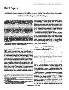
Figure 1: Learning curve (macro F1) (left) and number of sup-
0.300 0.275 0.250 0.225 0.200 0.175 0.150
0.0 0 0.0 01 0 0.0 02 0 0.0 03 0 0.0 04 0 0.0 07 0 0.0 12 0 0.0 19 0 0.0 32 0 0.0 52 0 0.0 85 1 0.0 39 2 0.0 28 3 0.0 73 61 1 0.1
port vectors (right)
2.0 4.0 8.0 16.0 32.0 64.0 128.0 256.0 512.0 1024.0 2048.0 4096.0 8192.0 16384.0 32768.0
Validation accuracy
γ
4
Analysis
The left axis of figure 1 shows how the performance changes as a function of the number of examples used. This graph uses the parameter settings and class weights from the main submission (i.e |V |=3000, C=51.79, γ=0.01). The lower curve (green) shows the mean and standard deviation of the official score for test sets selected by crossvalidation. The upper curve (red) shows performance on the (cross-validated) training set, which is always at ceiling. The right axis corresponds to the blue curve in the middle of figure 1 and indicates the number of support vectors used for various sizes of training set. Almost every added example is being catered for by a new support vector, suggesting overfitting. There is just a little generalisation for the green class, almost none for the others. Figure 2 shows the variation in macro-F1 with C and γ. The scoring function for grid search is the official macro-averaged F1 restricted to non-green classes, in contrast to the average accuracy used elsewhere. The optimal value selected by this cross-validation is C=64 and γ=0.0085. This is roughly the same as C=51.79, γ=0.01 chosen by cross-validation on average accuracy.
5
Discussion
The ReachOut challenge is evidently a difficult problem. The combination of class imbalance and an official evaluation metric that is very sensitive to performance on sparsely inhabited classes means that the overall results are likely to be unstable. It is not obvious what metric is the best fit for the
141
0.125 0.100
Figure 2: Heat map of variation of macro-F1 as a function of γ and C (with |V |=3000)
therapeutic application, because the costs of misclassification, while clearly non-uniform, are difficult to estimate, and the rare classes are intuitively important. It would take a detailed clinical outcome study to determine exactly what the tradeoffs are between false positives, false negatives and misclassifications within the positive classes. The labeled data set, while of decent size, and representative of what can reasonably be done by annotators in a small amount of time, is not so large that the SVM-based approach, with the features used, has reached its potential. The use of the class weight vector does appear to be helpful in improving the official score by trading off performance on the red label against a small loss of performance on the green label.
Acknowledgments Thanks to Tim Nugent for advice on understanding and visualizing SVM performance, and to Jochen Leidner and Khalid-Al-Kofahi for providing resources, support and encouragement. Thanks to all members of the London team for feedback and writing help.
References Chih-Chung Chang and Chih-Jen Lin. 2011. LIBSVM: A library for support vector machines. ACM Transactions on Intelligent Systems and Technology, 2:27:1– 27:27. Software available at http://www.csie. ntu.edu.tw/˜cjlin/libsvm. J. Gorodkin. 2004. Comparing two K-category assignments by a K-category correlation coefficient. Computational Biology and Chemistry, 28:367374. Stefan Knerr, L´eon Personnaz, and G´erard Dreyfus. 1990. Single-layer learning revisited: a stepwise procedure for building and training a neural network. In Neurocomputing, pages 41–50. Springer. Wes McKinney. 2010. Data structures for statistical computing in python. In St´efan van der Walt and Jarrod Millman, editors, Proceedings of the 9th Python in Science Conference, pages 51 – 56. F. Pedregosa, G. Varoquaux, A. Gramfort, V. Michel, B. Thirion, O. Grisel, M. Blondel, P. Prettenhofer, R. Weiss, V. Dubourg, J. Vanderplas, A. Passos, D. Cournapeau, M. Brucher, M. Perrot, and E. Duchesnay. 2011. Scikit-learn: Machine learning in Python. Journal of Machine Learning Research, 12:2825– 2830. David Vaughn and Derek Justice. 2015. On the direct maximization of quadratic weighted kappa. CoRR, abs/1509.07107.
142