Cluster Performance and the Implications for Distributed, Heterogeneous Grid Performance Craig Lee1
Cheryl DeMatteis1
James Stepanek1
Johnson Wang2
1
Computer Systems Research Department, M1-102 2 Fluid Mechanics Department, M4-965 The Aerospace Corporation, P.O. Box 92957, El Segundo, CA 90009-2957 {lee|cdematt|stepanek}@aero.org
[email protected]
Abstract This paper examines the issues surrounding efficient execution in heterogeneous grid environments. The performance of a Linux cluster and a parallel supercomputer is initially compared using both benchmarks and an application. With an understanding of how benchmark and application performance is affected by processor and interconnect speed, a comparison is made with the bandwidth and latencies available in a grid testbed. Of significant concern is the fact that the available communication bandwidth and latencies have a dynamic range of 3 to 4 orders of magnitude while processor speeds have a range of about one half order of magnitude. Also, while both processor speed and network bandwidth are increasing very rapidly, simple propagation delay will become more significant in the network latencies seen by many grid applications. That is to say, the pipes in a grid will be getting fatter but not commensurately shorter. How are we to effectively utilize such an infrastructure? Clearly an attractive approach is to require sufficient concurrency in the application such that a coarsegrain, data-driven model of execution can be used to hide latencies while hopefully keeping context switching overheads low. If the “spatial component” of an application is understood, then runtime systems could also apply established techniques like caching, compression, estimation and speculative pre-fetching. Ideally this low-level performance management should be encapsulated in an easy-to-use abstraction.
1 Introduction Cluster computing has been gaining wide acceptance over single-machine, massively parallel computing due to
its undeniable cost-effectiveness for suitable applications [4]. Since clusters are built from commodity hardware, however, they typically have slightly slower processors and lower communication bandwidths than “big iron” machines. Hence, suitability in this context means simply that either (1) an application must be more tolerant of higher communication costs, or (2) the user’s “mission requirements” are lenient enough to accept the lower performance at a much lower dollar cost. The increasing potential of grid computing, however, means that users and applications will be faced with environments that have an even greater heterogeneity of communication abilities. [8]. While this potential includes the flexible harnessing of resources on a scale not previously considered for individual applications, it also means that achieving efficient use of those resources will be harder than ever. This paper endeavors not to present any solutions to this problem but to quantitatively demonstrate the bounds of the problem as motivation for exploring candidate programming and execution models that can effectively operate in a grid environment. We will do this by comparing the performance of a parallel machine, a cluster, and a grid testbed by several means. These are specifically the Cray T3E [13], a Pentium cluster with fast ethernet, and the Globus GUSTO testbed [7], which are representative of their respective classes. (Different examples of each class could be used but the fundamental relationships between them would not be altered.) The Cray T3E used here is the T3E-1200 at the CEWES Major Shared Resource Center in Vicksburg, Mississippi. It has 512 DEC Alpha 21164 processors clocked at 600 MHz. with 128 MB of memory per processor. Its 3D torus dedicated interconnect is capable of 650 MB/sec. (theoretical peak) in both directions. The cluster used here is at the Aerospace Corporation. It has fourteen Intel Pentium
II processors clocked at 400 MHz. running Red Hat Linux with 192 MB of memory per processor. They are connected by 100 Mbit/sec. fast ethernet through a Baystack 450-24T switched ethernet hub. The Globus GUSTO testbed is distributed across many adminstative sites and includes a large variety of machines. The current configuration of GUSTO can always be examined by using the Metacomputing Directory Service (MDS) Browser on the Globus web site (www.globus.org). These “machines” (including the grid) will be compared using parallel benchmarks, a parallel application, and a distributed performance monitoring tool. We will look at the relative processing speeds and communication speeds. We then discuss the implications of achieving efficiency in an increasingly heterogeneous computing infrastructure.
2 A Benchmark Comparison To compare the performance of a Linux cluster and a parallel supercomputer, we use the NAS Parallel Benchmarks [12]. These benchmarks were developed by the Numerical Aerodynamics Simulation (NAS) group at NASA Ames with the goal of being able to make more reliable quantitative performance comparisons among parallel machines. These benchmarks consist of numerical kernels for a wide range of computing problems. Rather than a single “microbenchmark” that may exercise only one aspect of a machine, these benchmarks were chosen to exercise all aspects of a machine, individually and in combination. Specifically these benchmarks exercise communication, integer computation and floating-point computation. For brevity and conciseness, we only need to present the results of two benchmarks that illustrate the major difference between these two platforms. For each benchmark, the per processor performance is plotted as a function of the number of nodes. These two benchmarks involve integer computation, so the measurement metric is millions of operations per second per node: Mop/sec/node. This allows the relative performance and scalability on each platform to be shown in one graph. For each benchmark, there are also three classes, A, B, and C, that correlate to three different problem sizes, with A being the smallest and C being the largest. Hence, for each benchmark graph, there are three curves (one for each class) for both platforms. For consistency and ease of comparison, the same point symbol is used for each platform. The same line style is used for each benchmark class. Figure 1 shows the Random Number Generation benchmark. This is an “embarrassingly parallel” benchmark since the parallel tasks (generating random numbers) are completely independent, i.e., after the tasks are started, there is absolutely no communication or synchronization between nodes. As expected, both platforms show good scaling (flat
curves). The Alpha processors, however, are approximately 4x faster than the Pentium IIs. Figure 2 shows the Integer Sorting benchmark. Integer sorting is not a computationally complex task since it primarily requires the comparison of integers. It can, however, require massive amounts of communication as data values are relocated to their sorted positions. Here we see that the T3E exhibits not only faster processing but also much better communication scaling. For the cluster, the per-node performance falls off dramatically as the number of nodes increases. These two benchmarks dramatically illustrate the performance differences between parallel and distributed computations that are compute-bound versus communicationbound. In the sorting benchmark, the communication bandwidth is clearly dominating the overall performance. In terms of relative performance and scalability, the other NAS Parallel Benchmarks fall inbetween these two extremes.
3 An Application Comparison In this section, we use an application to compare the performance of these two platforms. That application is ALSINS (Aerospace Launch Systems Implicit NavierStokes), a computational fluid dynamics (CFD) code developed by the Fluid Mechanics Department at Aerospace and used to investigate flow fields of the Delta-II and Titan-IV launch vehicles [16, 15]. CFD works by discretizing the space around a physical object into “cells” and computing the flux of material between cells by solving the Navier-Stokes equations for a sequence of time steps until the solution has converged to a final state. CFD is typically parallelized by decomposing the discretized spatial domain and assigning different blocks to different processors. The algorithm has an iterative structure consisting of (1) exchanging neighbor data, (2) computing the minimum time step among all blocks, and (3) computing the flux for the current time step. For ALSINS, this is implemented using MPI. With this basic structure, there are two hard synchronizations per iteration: exchanging neighbor data and the minimum time reduction. Aside from potential synchronization delays, the minimum time reduction is a very quick operation since it only involves finding the minimum of a single floating-point time step value across all nodes. The time required for communication and the local flux computation, however, depends on the data block size allocated to each node. Note that it is possible to improve efficiency by overlapping communication and computation for a given iteration. The rate of convergence for the solution depends on the geometry of the test case and can be on the order of 105 iterations. The speed at which iterations can be computed depends on the total size of the discretized space and
Random Number Generation 10
Mop/sec/node
"t3e.ep.A.mops" "t3e.ep.B.mops" "t3e.ep.C.mops" "beo.ep.A.mops" "beo.ep.B.mops" "beo.ep.C.mops"
1
0.1 0
5
10 number of nodes
15
20
Figure 1. The Random Number Generation Benchmark. Integer Sorting 10
Mop/sec/node
"t3e.is.A.mops" "t3e.is.B.mops" "t3e.is.C.mops" "beo.is.A.mops" "beo.is.B.mops"
1
0.1 0
5
10 number of nodes
15
Figure 2. The Integer Sorting Benchmark.
20
the number and speed of the processing nodes used on the problem. The test case computed using ALSINS is the flow field around the base of a Centaur launch vehicle with both engines running with exhaust plumes. Figure 3 shows a flow field computation done on the Pentium cluster. ALSINS performance was measured and analyzed using NetLogger [14], a tool developed at Lawrence Berkeley Lab for analyzing distributed systems. NetLogger logs timestamped, application-defined events either locally or to a remote logging daemon. The NetLogger visualization tool, nlv, can subsequently display these events as grouped, color-coded sets of events, called lifelines, over time. Other events or statistics associated with a scalar values, such as cpu load, can be also be displayed as loadlines. ALSINS with the Centaur Double Nozzle test case was run on both platforms in two versions using overlapped and non-overlapped communication. The NetLogger visualization display for two representative iterations of the overlapped code version on the Pentium cluster is shown in Figure 4. This shows the color-coded, per-iteration lifelines for each node. Each lifeline consists of six events tags: REDUCE TAU, START COMM, START SOLVER, SOLVER DONE, COMM DONE, and COPIES DONE. Loadlines for the utilization (number of processors actively engaged in communication or computation) and the efficiency (utilization over the duration of the computation) are also shown. These results show us that per iteration, ALSINS is ≈2.9x faster on the T3E than on the cluster (4.75 seconds vs. 1.63 seconds). Part of this difference is due to the faster processors on the T3E and also a memory subsystem augmented with stream buffers. Of this iteration time, however, there is ≈19% idle time due to the load imbalance. Hence, there is an efficiency of ≈81% where processors are busy doing communication or computation. On the cluster, communication takes ≈16% of the iteration time. On the T3E, communication takes ≈2%.
4 A Bandwidth µbenchmark Comparison It is certainly not news that communication bandwidth plays a direct role in determining parallel application performance. But in the scope of emerging computational infrastructures, however, what is the depth of the communication hierarchy? What is the range of impact that communication infrastructures can have, will have, on distributed, parallel applications? We examine this question in two parts. First, we do a simple MPI bandwidth test between the Pentium cluster and the T3E. Second, we compare these results with a histogram of host pair bandwidths on the Globus GUSTO testbed [7]. The MPI bandwidth test program we used tests a variety
of communication patterns with differing number of nodes and different data volumes (message sizes). We ran this program on both the Pentium cluster and the T3E. For brevity and conciseness, we present only the most relevant data in Table 1. In this particular test, bidirectional communication occurs among all nodes simultaneously for two to eight nodes. This means that every node is sending and receiving a 1 MB message from all other nodes at the same time to stress the limits of performance. The cluster is theoretically capable of 100 Mbit/sec. or 12.5 MB/sec. For two nodes, a bidirectional bandwidth of over 10 MB/sec., or 80 Mbit/sec., is achieved. This is the expected end-to-end result since overhead in the messagepassing process, e.g., buffer copying and device driver scheduling, etc., means that an application will always see less bandwidth than the physical medium is “clocked” at; in this case, fast ethernet. Note, however, that as more nodes are added to the test, the realized bandwidth sinks to about 4 MB/sec. This indicates that contention for resources is occurring somewhere. (While the hub is technically nonblocking, it may still have a backplane that is becoming saturated as the aggregate bandwidth demand increases.) For the T3E, we see that two nodes are capable of over 300 MB/sec. For eight nodes, the average bidirectional bandwidth is still over 200 MB/sec. This means that the dedicated communication hardware on the T3E is 30x to 50x faster than fast ethernet in a cluster. (This might lead one to conclude that much of a large machine’s cost is in its dedicated interconnect.) How do these bandwidths compare with that typically available in a grid environment? To answer this question, we made use of the Gloperf network performance data that is periodically uploaded into the Globus Metacomputing Directory Service (MDS) [6]. The MDS is based on the Lightweight Directory Access Protocol (LDAP) and provides an information naming scheme and repository for all manner of grid computing information, e.g., available hosts, number of nodes, current load, network interfaces, gatekeeper contact information, etc. It is also used to record bandwidth and latency data periodically measured between host pairs by Gloperf. Gloperf [10] is a simple tool that is automatically deployed on each Globus host. At Globus boot-time, the Gloperf daemon will register itself in the MDS and then query the MDS for all other Gloperf daemons. The daemon will then make periodic bandwidth and latency tests with all other daemons and store the results in the MDS. (The initial implementation of Gloperf did measurements between all pairs which does, of course, result in non-scalable behavior. The latest implementation uses a simple group scheme to produce hierarchies of measurements.) The actual Gloperf measurement mechanism is borrowed from netperf. Gloperf is configured to perform a
Figure 3. The Centaur Double Nozzle Test Case Computed on a Pentium Cluster.
Figure 4. ALSINS with overlapped communication/computation on the Pentium Cluster.
Cluster Bandwidth, MB/sec. Avg. Node 0 Node 1 10.348 10.379 10.317 8.076 10.225 6.957 8.730 10.028 7.561 7.869 9.979 7.941 6.472 6.689 6.216 6.778 8.355 7.276 4.489 6.072 4.907 T3E Bandwidth, MB/sec. Avg. Node 0 Node 1 319.252 319.101 319.402 253.973 253.161 253.259 224.496 218.161 211.452 194.584 194.335 190.279 203.172 215.007 181.744 222.200 231.971 193.002 211.705 212.216 191.008
Node 2
Node 3
Node 4
Node 5
Node 6
Node 7
7.047 9.910 6.675 7.035 6.483 4.948
7.421 8.135 6.207 5.868 4.426
6.616 6.354 7.194 4.167
6.333 6.445 3.942
5.822 3.727
3.726
Node 2
Node 3
Node 4
Node 5
Node 6
Node 7
255.498 241.411 219.954 242.082 282.610 236.182
226.958 183.446 184.683 198.681 200.079
184.905 213.967 238.679 235.900
181.548 217.750 222.200
192.702 205.023
191.024
Table 1. Bandwidth tests for T3E and Cluster.
10-second, TCP “packet-blasting” test and measure the data volume sent. Gloperf also measures the number round-trips that can be made in a 10-second period. The sequence of hosts and test types (bandwidth and latency) are randomized in order. Since Gloperf does untuned TCP testing from the user-level, it essentially observes the same end-to-end performance that an application would see. To extract the Gloperf data from the MDS, a simple program would periodically snapshot the MDS Gloperf data into log files. Scripts were then used to extract just the bandwidth and latency data and eliminate duplicates. Figure 5 shows histograms of Gloperf bandwidth and latency measurements on GUSTO beginning in August and continuing through October, 1999. This represents 18615 unique measurements between 3405 unique host pairs over 138 unique hosts; mostly in North America but including a few in Europe, Asia, and Australia. Note that these histograms employ log-sized bins that make the mode of the distributions much more evident. While it was not uncommon to observe bandwidths as high as 96 Mbits/sec., the median bandwidth for this distribution is 2.2 Mbits/sec. and the 90th percentile is 15.1 Mbits/sec. While the latency distribution has a much narrower (rhinokurtotic) mode, common latencies span three orders of magnitude. Here, the median is 57.35 msec. and 90% of the latencies are above 5.5 msec. It is clear that in a grid environment that can include clusters and “big iron” machines, there can be a 3 to 4 order of magnitude dynamic range in the bandwidth and latencies available to an application.
5 Discussion and Implications What are the implications of these observations for heterogeneous cluster performance and grid performance? The argument can be made that there is a much greater dynamic range in the the available communication bandwidths than there is in processor speeds; 3 to 4 orders of magnitude versus one half order of magnitude. We note that since the graphs in Figure 5 represent capacity that is shared among other non-Globus traffic, one could argue that in terms of a shared resource, processors could exhibit the same range of available cycles. A counter-argument, however, is that one typically has greater control over the compute resources rather than the network; even if one does not have complete control of the processors, the processors may be batch scheduled. Regardless of such arguments, in many cases there will be a significant differential between the available processor speeds and network speeds. What is the implication of this processor-network differential? We note that processor speeds have been increasing according to Moore’s Law (doubling every 18 months). Memory bandwidth, however, has been increasing much more slowly, by some estimates as little as 7% per year. To cope with this processor-memory differential, hardware designers have had use increasingly larger caches and to employ numerous techniques to overlap operations to hide latency, such as speculative execution, prefetching, and hardware multithreading. This has also motivated the research in Processing-In-Memory (PIM) architectures [9]
1400 1200
count
1000 800 600 400 200 0 0.0001
0.001
0.01 0.1 1 10 bandwidth (Mbits/s), 100 log-sized bins
100
1000
2500
2000
count
1500
1000
500
0 0.1
1
10 100 latency (ms), 100 log-sized bins
1000
Figure 5. Globus testbed bandwidth and latency distributions.
10000
where much higher bandwidths between memory and the processing units can be realized. Fortunately network bandwidths seem to be increasing at least as fast as Moore’s Law, if not faster, since around 1994 (A.W. – After Web). Unfortunately this improvement in bandwidth will not affect the speed of light. A significant part of latencies present in a grid is simply propagation delay. As an example, the end-to-end, application-level message-passing latency between Los Angeles and Chicago can already be as much as 33% propagation delay. Clearly this limits the reduction in latencies that are physically possible in a grid computing environment. Hence, in ten years time, we might expect the bandwidth distribution in Figure 5 to move to the right by an order of magnitude. While the possible relative reduction in latency will depend on the geographic separation among the compute resources, it is safe to say that many latencies in the latency distribution will not decrease as much. The bottom-line is that pipes will get fatter but not commensurately shorter. How exactly will this relative change in bandwidths, latencies and processing speeds affect application performance? Work done by Martin, et al., is relevant to this question [11]. They examined the effect of latency, overhead and bandwidth on cluster performance. For this work, latency is defined as the end-to-end delay in sending a message from its source to its destination. Overhead is defined as the time that a processor is engaged in message transmission or receipt during which it cannot do anything else. Bandwidth is inversely defined in terms of the “gap” between consecutive message sends, i.e., messages per unit time. For a set of applications on an UltraSPARC cluster using Myrinet A set of applications were run on an UltraSPARC cluster using Myrinet where the LANai processor on the Myricom network interface card was used to emulate a range of latencies, bandwidths and overhead. The applications in this experimental context were much more sensitive to overhead than to bandwidth or latency. For these applications, one is forced to conclude that since the additional per message overhead was unavoidable, it directly affected the application’s running time, while at least part of the additional latency was naturally overlapped or hidden by the structure of the application. It was also shown that the applications had relatively modest bandwidth requirements compared to the dedicated network’s capacity. Most applications did not slow-down significantly until the bandwidth was effectively reduced to approximately 12% of its normal capacity. Indeed, even the increased latencies in this cluster were well below those found in a grid and the reduced bandwidths were above the 90th percentile. In a general grid environment, these results would be different. In the light of these considerations, the next question to ask is “How tightly coupled do distributed, heterogeneous grid applications need to be or can be?” Clearly not all ap-
plications are tightly coupled or need to be, in the sense that a CFD code is tightly coupled. Applications that connect unique resources, such as X-ray sources, with visualization devices, such as CAVEs, typically rely on a functional decomposition that is more tolerant of the dynamic range of bandwidth within a machine and between machines. Nonetheless, all distributed applications will run better with faster networks. This is not news. In the context of the World Wide Web, most people probably feel that downloads are too slow. In part, the notion of quality of service is to provide a “floor” to the performance that a user receives from a shared resource, e.g., a network. The opinion is also held that flexibility is actually more important for grid applications than performance management. For a large class of applications, this will be true. The grid is being designed to make it as easy as possible to compose disparate resources such as specialized databases, unique instruments, and embedded systems. For another large class of applications, however, the grid holds the promise of applying very large amounts of aggregate compute power to very large problems that is not economically feasible any other way. Hence, what can be done to manage performance across these bandwidths and latencies? Cluster computing can, again, be used as a point of departure. Several projects have been reported that deal with programming clusters of SMPs, or clumps, where the heterogeneity of in-memory communication vs. network communication is the central issue. The SIMPLE model [2], for example, provides a simple set of collective operations that are handled by different modules for intra-node and internode communication. KeLP and its Data Mover [5, 1] take a different approach. KeLP defines a set of meta-data abstractions, such as Region, Map, FloorPlan and MotionPlan, that capture the geometry of block-structured decomposition and the resulting data dependencies in parallel execution. The current Data Mover implementation uses a private MPI communicator and asynchronous pointto-point messages to actually move the data. An important issue for communication libraries or runtime systems that support higher-level semantics, however, is that of irregular communication; communication that does not follow a regular, geometric pattern and may be dynamic and not known until run-time. This issue has been faced by the High Performance Fortran (HPF) community for some time. This has given rise to an inspector-executor paradigm where an inspector routine does a run-time analysis of array accesses for communication and derives a communication schedule that is then used by the executor routine to actually perform the communication. Since the inspector routine can be very time-consuming, there has been work done on minimizing its overhead and reusing any schedules produced [3]. For some applications, it will be best to use a program-
ming model that does not hide the heterogeneity of the underlying resources and requires the application builder to hand-code the application to the resources. There are, of course, great benefits in not having to hand-code applications to tolerate bandwidths and latencies. For these situations, dealing with a heterogeneous infrastructure means addressing the fundamental problems of (1) data locality and (2) scheduling, where scheduling in this context means both communication and execution scheduling which are, in fact, interdependent. A clearly attractive approach is to require sufficient concurrency in the application such that a coarsegrain, data-driven model of execution can be used. The initial challenge is to hide latency with concurrency while keeping context switching overheads low. The next challenge is to encapsulate this low-level performance management into an easy-to-use package or component. If this is possible, then other established techniques such as caching, compression, estimation and speculative pre-fetching, could also be used. Finally we note that applications tend to have their own, natural “problem architecture” and some, by their very nature, are more tightly coupled than others. As soon as a distributed implementation is considered, it imparts a threedimensional or spatial “density distribution” to the computation. This density and the available bandwidth and latency become part of the algorithmic complexity governing performance. Some applications will have unavoidable spatial constraints that will be best addressed by recasting the problem and its solution in a more loosely coupled fashion. The Barnes-Hut algorithm, for example, solves the N-Body problem in less than O(n2 ) complexity by representing space with an octree such that from any given body, groups of far away bodies can be represented as a point source. The challenge for grids and heterogeneous computing, however, is to minimize the class of applications that have to be recast by developing systems and runtimes that understand the “spatial component” of an application and can act accordingly to provide the best overall performance with the available communication resources. This is one of the goals of the Grid Forum’s Advanced Programming Models Working Group (www.gridforum.org). The need for such “spatial component” management will only increase as systems like long-latency satellite networks and low-power mobile networks come online with high-performance compute systems such as hardware multithreaded processors that tolerate deep memory hierarchies.
References [1] S. Baden and S. Fink. The Data Mover: A machineindependent abstraction for managing customized data motion. LCPC, August 1999.
[2] D. Bader and J. JaJa. SIMPLE: A methodology for programming high performance algorithms on clusters of symmetric multiprocessors. Technical report, University of Maryland, Department of Computer Science, and The University of Maryland Institute for Advanced Computer Studies, 1997. Tech report, CS-TR-3798, UMIACS-TR-97-48. [3] S. Benkner, P. Mehrotra, J. V. Rosendale, and H. Zima. High-level management of communication schedules in HPF-like languages. International Conference on Supercomputing, 1998. [4] CESDIS. The Beowulf Project. Technical report, NASA, 1999. http://www.beowulf.org. [5] S. Fink and S. Baden. Runtime support for multitier programming of block-structured applications on smp clusters. International Scientific Computing in Object-Oriented Parallel Environments Conference (ISCOPE ’97), December 1997. Available at wwwcse.ucsd.edu/groups/hpcl/scg/kelp/pubs.html. [6] S. Fitzgerald, I. Foster, C. Kesselman, G. von Laszewski, W. Smith, and S. Tuecke. A directory service for configuring high-performance distributed computations. In Proceedings 6th IEEE Symp. on High Performance Distributed Computing, pages 365–375, 1997. [7] I. Foster and C. Kesselman. Globus: A metacomputing infrastructure toolkit. Intl. J. Supercomputing Applications, 11(2):115–128, 1997. [8] I. Foster and C. Kesselman. The Grid: Blueprint for a New Computing Infrastructure. Morgan Kaufmann, 1998. [9] M. Hall et al. Mapping irregular applications to DIVA, a PIM-based data-intensive architecture. Supercomputing ‘99, 1999. [10] C. Lee, R. Wolski, J. Stepanek, C. Kesselman, and I. Foster. A network performance tool for grid environments. Supercomputing ‘99, 1999. [11] R. Martin, A. Vahdat, D. Culler, and T. Anderson. Effects of communication latency, overhead, and bandwidth in a cluster architecture. 24th ISCA, June 1997. [12] NAS. The NAS Parallel Benchmarks. Technical report, NASA, 1999. http://www.nas.nasa.gov/Software/NPB/index.html. [13] SGI. The Cray T3E Homepage. Technical report, SGI, 1999. http://www.sgi.com/t3e. [14] B. L. Tierney. NetLogger: A methodology for monitoring and analysis of distributed systems. Technical report, Lawrence Berkeley Laboratory, 1999. http://wwwdidc.lbl.gov/NetLogger. [15] J. Wang and S. Taylor. Industrial Strength Parallel Computing, chapter 10: An architecture-independent Navier-Stokes Code. Morgan Kaufman, Inc., 1999. [16] J. Wang and G. Widhopf. An efficient finite volume TVD scheme for steady state solution of the 3-D compressible Euler/Navier-Stokes equations. In AIAA paper 90-1523, June 1990.