1
Performance Implications of Failures in Large-Scale Cluster Scheduling Yanyong Zhang Department of Electrical and Computer Engineering Rutgers University Piscataway, NJ 08854
[email protected]
Mark S. Squillante Mathematical Sciences Department IBM T.J. Watson Research Center Yorktown Heights, NY 10598-0218
[email protected]
Anand Sivasubramaniam Department of Computer Science and Engineering Pennsylvania State University University Park, PA 16802-6106 Email:
[email protected]
Ramendra K. Sahoo Exploratory Server Systems Department IBM T.J. Watson Research Center Yorktown Heights, NY 10598-0218
[email protected]
Abstract— As we continue to evolve into large-scale parallel systems, many of them employing hundreds of computing engines to take on mission-critical roles, it is crucial to design those systems anticipating and accommodating the occurrence of failures. Failures become a commonplace feature of such large-scale systems, and one cannot continue to treat them as an exception. Despite the current and increasing importance of failures in these systems, our understanding of the performance impact of these critical issues on parallel computing environments is extremely limited. In this paper we develop a general failure modeling framework based on recent results from large-scale clusters and then we exploit this framework to conduct a detailed performance analysis of the impact of failures on system performance for a wide range of scheduling policies. Our results demonstrate that such failures can have a significant impact on the mean job response time and mean job slowdown under existing scheduling policies that ignore failures. We therefore investigate different scheduling mechanisms and policies to address these performance issues. Our results show that periodic checkpointing of jobs seems to do little to ease this problem. On the other hand, we demonstrate that information about the spatial and temporal correlation of failure occurrences can be very useful in designing a scheduling (job allocation) strategy to enhance system performance, with the former providing the greatest benefits.
I. I NTRODUCTION Our growing reliance on computing and information processing services mandates not only deploying systems that can meet the performance demands imposed on such systems, but also those that are available when needed. Several technological factors are accentuating the problem of system failures, which are highly undesirable since these systems could be servicing the needs of hundreds of users. At the same time, solutions for this problem need to keep the high costs of system maintenance personnel in mind, which is growing to be a much more important factor in Total Cost of Ownership (TCO). A deep understanding of the occurrence of failures in real environments can be useful in several ways towards enhancing overall system availability. It can provide realistic data when evaluating proposed solutions, together with developing strategies for proactive prediction and remedies of faults ahead of their occurrence. Application demand for high performance is continuing to fuel research and development of large scale parallel systems. The need for processing larger datasets in existing applications, and the stringent demands of emerging applications necessitate par-
allelism in computational and storage devices for their deployment. The cost-effectiveness in using off-the-shelf hardware to put together clusters has contributed to a large extent in the widespread availability of parallelism, and its successful usage. At the same time, several important and challenging applications are driving the development of large scale parallel machines, such as IBM’s BlueGene/L which is anticipated to have 65536 nodes. As we continue to develop such large scale parallel systems, there are several important technological factors to keep in mind: •
•
•
Denser integration of semiconductor circuits, though preferable for performance, makes them more susceptible to strikes by alpha particles and cosmic rays [41]. At the same time, there is an increasing tendency to lower operating voltages in order to reduce power consumption. Such reduction in voltage levels can increase the likelihood of bit-flips when circuits are bombarded by cosmic rays and other particles, leading to transient errors. While memory structures are typically the target for protection against errors using informational redundancy, more recent studies [31] have pointed out that the error rates in combinational circuits are likely to surpass those of memory cells in the next decade. At the macro granularity, we have dense bladesystems being packed in a rack as a cluster. With a high load imposed on these dense systems – both on the CPUs and on the disks – heat dissipation becomes a very important concern, potentially leading to thermal instability that can cause system/node breakdowns [25], [9]. We find system software and applications becoming more complex. Such complexity makes them more prone to bugs and other software failures [35], [23], [38] (e.g. memory leaks, state corruption, etc.). These bugs/failures can cause system crashes, and it has even been suggested that one should per-
2
form pro-active shutdown/rejuvenation [39], [38] to avoid catastrophic consequences.
All these factors point to the increasing occurrence of system failures in the future. Failures become more commonplace when we consider parallel systems with thousands of nodes. Rather than treat them as an exception, system design needs to recognize fault occurrence, and manage the resources across the parallel system effectively so as to hide their impact from the end users. One would ideally like to achieve the performance of a system without any failures. Even if this is difficult to attain, there should be at most a “graceful degradation” in performance under the presence of failures. Towards this goal, the present paper specifically targets the management of CPU resources on a large scale parallel system using a general failure modeling framework that accurately represents the node failure characteristics reported in recent studies of extensive error logs collected from cluster systems over long periods. When nodes1 fail, there are two important consequences on system performance: •
•
First, the process/task of the application running on this node dies, consequently loosing all its work since it began. Further, in a parallel application, tasks frequently communicate and consequently other tasks would also not be able to progress. In effect, this can cause restarting the entire application (either on the same nodes or on different nodes). Second, the unavailability of the failed node can cause longer queueing delays for waiting jobs.
In this paper, we focus mainly on the first issue. With transient hardware errors and software errors expected to be more prevalent than permanent failures, node reboots/restarts can fix many of these problems. The duration of unavailability would then 1
Since we are mainly concerned with CPU management, we use the terms, node and CPU, interchangeably in the rest of the paper.
be relatively low, given the long execution times of many of the parallel applications that we are targeting – those in the scientific domain at national laboratories and supercomputing centers. Note that the impact of node recovery time can become quite important for permanent failures, and we postpone such an investigation for future work. There are several options for managing the nodes in a faulty environment. One could use an optimistic approach, and simply ignore the problem, assuming there would be no failures. When a node does fail, then the application (all its tasks) could be restarted as was just explained. However, as our results will show, such an approach can suffer significant performance loss compared to a system where there is no failure. At the other end of the spectrum, we could have a more pessimistic strategy, where application processes are periodically checkpointed so that when a fault occurs, the amount of work to be re-done is limited. In our results we will show that while this can be better than ignoring the problem, the overheads of checkpointing can limit its benefits. In this paper, we investigate an alternative strategy whose main philosophy is that if we have a better idea of when and where failures occur, then one could use such information for better management of the CPUs: •
•
If we could predict the time for the failure, then we could checkpoint immediately before this point in time, so that we significantly limit the work lost while reducing the checkpoint overheads. However, it may be very difficult to predict the exact time for failures. If, on the other hand, temporal prediction of failures is possible with a coarser granularity (a window) [29], then checkpointing could be initiated only within those windows. If we could predict the nodes (spatial prediction) that fail, then we could either avoid scheduling jobs on those nodes as far as possible, or only checkpoint those nodes. The latter option may not be very fruitful since parallel
3
applications typically require all tasks to make progress at around the same rate. One could also use a combination of spatial and temporal prediction to specifically focus on the time and nodes where pro-active action needs to be taken to limit the work loss upon failure while limiting the overheads of checkpointing. Investigation of these alternatives requires an understanding of the failure characteristics of real parallel systems executing parallel applications. Unfortunately, the research literature provides a wide variety of often conflicting results for different computing environments (hardware and software) and there seems to be a lack of consistent conclusions in previous computer failure studies. Moreover, only a few recent studies have even considered large-scale clusters and they have tended to focus on sequential commercial applications. The only exception that we are aware of is a recent study [28] of extensive error logs collected from a large-scale distributed system consisting of close to 400 machines over a period of close to 500 days, which includes some parallel applications. We therefore develop a general modeling framework that makes it possible to vary the properties of the failure patterns to span the wide range of failure characteristics found in the research literature. This framework is exploited to understand the impact of different failure characteristics on overall system performance and to propose scheduling strategies that can alleviate the performance impact of different failure attributes. A detailed simulation study using this failure modeling framework and characterized parallel job workloads from a supercomputing center reveals that the failures do account for a significant drop in performance compared to a system without failures. As can be expected, an exact temporal prediction of node failures almost completely bridges this gap of performance loss due to failures. Our results also show that a significant portion of this gap can be bridged even if temporal prediction can be done at only a granularity of 2–4 hours. While the results from our statistical analysis demonstrate clear
patterns that could be exploited to provide such coarse grain temporal prediction, the results of our simulation study further show that even greater performance benefits are possible by using the spatial (node) behavior of failures. Hence, our solution opts to exploit the statistical spatial properties of failures and does so by developing a scheduling strategy wherein nodes that have recently failed are given lower priority at being assigned a job compared to others. We demonstrate that this simple strategy suffices to extract most of the performance gap between a system with failures and one without, and does significantly better than blindly checkpointing at periodic intervals. The rest of this paper is organized as follows. The next section provides a brief summary of work related to this study. Section 3 presents our evaluation methodology, including our system model, our failure modeling framework, and the performance metrics of interest. Simulation results of the impact of failures on system performance are provided in Section 4, followed by consideration of different failure-aware scheduling strategies in Section 5. II. R ELATED W ORK Job scheduling plays a critical role in the performance of large scale parallel systems (e.g. refer to [8], [43], [44], [10], [12], [16], [18], [32], [33], [34] and the references therein). At the same time, scheduling can be used to improve the faulttolerance [1], [27] of a system in three broad ways. First, a task can be replicated on multiple nodes so that even if a subset of these nodes fail, the execution of a task is not impacted. Studies that employ this technique ( [30], [17]) assume a probability for node failure to determine the number of nodes on which to replicate the task. Second, the system can checkpoint all the jobs periodically so that work loss is limited when a failure occurs, and there are several studies on tuning checkpoint parameters [21], [4], [22]. Third, the scheduler allocates spare nodes to a job so that it can quickly recover from potential failures [26].
4
With this approach there is a trade-off between using the extra node(s) to improve the response time versus time for recovery. To our knowledge, there has not been prior work in analyzing and possibly managing system resources based on node failures.
III. E VALUATION M ETHODOLOGY A. System Model We simulate a 320-node cluster that runs parallel workloads. A parallel job consists of multiple tasks, and each task needs to run on a different node. After certain nodes are allocated to a job, they are dedicated to the job until it completes (i.e., no other jobs can run on the same nodes). Multiple parallel jobs can run side by side on different nodes at the same time. After a job arrives, it will start execution if it is the first waiting job and the system has enough available nodes to accommodate it. Otherwise, it will be kept in the waiting queue. In this paper, all the waiting jobs are managed in the First-ComeFirst-Serve (FCFS) order. We also use backfilling in this exercise, which is a most commonly used scheduling technique [44] for parallel workloads. Backfilling allows a job that arrived later to start execution ahead of jobs that arrived earlier as long as its execution will not delay the start of those jobs. Estimated job execution times are required to implement backfilling. Our experiments use a workload that is drawn from a characterization of a real supercomputing environment at Lawrence Livermore National Labs. Job arrival, execution time and size information of this environment have been traced and characterized to fit a mathematical model (Hyper-Erlang distribution of common order). The reader is referred to [11] for details on this work and the use of the model in different evaluation exercises [44]. The workload model provides (1) arrival time, (2) execution time, and (3) size (number of nodes that it needs) for each incoming job.
B. Failure Injection A large number of studies have considered the characteristics of failures and their impact on performance across a wide variety of computer systems. Tang et al. [37], [36] and Buckley et al. [5], [6] have investigated error/failure logs collected from various VAXcluster systems of different sizes. Lee et al. [19] and Lin et al. [20] analyzed the error trends for Tandem systems and DCE environments. Xu et al. [40] performed a study of error logs collected from a heterogeneous distributed system consisting of 503 PC servers. Heath et al. [13] considered failure data from three different clustered servers, ranging from 18 workstations to 89 workstations. Castillo et al. [7], Iyer et al. [15] and Meyer et al. [24] have explored the effects of workload on different types of computer system failures. Vaidyanathan et al. [38] demonstrated that software-related error conditions will accumulate over time which will eventually lead to crashes/failures. Sahoo et al [28] have investigated the error logs from a networked environment of close to 400 heterogeneous servers over a period of close to 500 days. Many of these studies have identified statistical properties and proposed stochastic models to represent the failure characteristics of various computer systems. This includes the fitting of failure data to Weibull, lognormal and other specific distributions, each with different parameter settings, under the assumption of independent and identically distributed failures [20], [19], [13]. Other studies have demonstrated that the sequence of failures on some computer systems are correlated in various ways and that the failures tend to occur in bursts [37], [36], [40], [28]. Semi-Markov processes also have been proposed to model the time-series of failure from certain systems [14], [37], [36]. Unfortunately, only a few of these previous studies have even considered clustered server environments and those that have tend to focus on commercial servers like web servers, file servers and
5
database servers. We are not aware of any studies that investigate failures within the context of largescale clusters executing parallel applications, and no failure logs collected from such parallel computing environments are available to us. Moreover, given the wide variety of often conflicting results and the lack of consistent conclusions in previous computer failure studies, we expect that parallel computing environments with different parallel application workloads, system software and system hardware will similarly exhibit a broad range of failure behaviors. It is therefore important to have a general modeling framework that makes it possible to vary the properties of the failure patterns used to investigate parallel scheduling issues. Hence, we develop such a failure modeling framework in this section which is then exploited in Sections 4 and 5 to understand the impact of different failure characteristics on overall system performance and to propose scheduling strategies that can alleviate the performance impact of different failure attributes. Our framework consists of models for each of the three primary dimensions of failure characteristics together with controls over each of these dimensions and their interactions. The first dimension concerns the times at which failures occur. This includes the marginal distribution for the time between failures as well as any correlation structure among the individual failures. The second dimension concerns the assignment of failures among the nodes comprising the system. This allows our framework to span the range from uniformly distributed node failures assumed in some previous failure studies to strong correlations between failures and nodes in order to yield the types of concentrations of failures on a subset of nodes as demonstrated in several recent failure studies of large-scale clusters. The third dimension concerns the down time of each failure. An overall control model is also used to directly capture any correlations or interactions among these three dimensions. Thus, there is no loss of generality in separating out the individual dimensions, while providing the
ability to explicitly control and vary each aspect of the individual dimensions. We now define the specific aspects of each dimension of our general failure modeling framework that are used in this study to generate synthetic failure workload traces each consisting of a number of failures. We use the job workload duration to determine the total number of failures (F ) by making sure that the failures are spread throughout the entire span of parallel job executions. a) Time of failures.: Let ti denote the time at which failure i occurs, i = 1, . . . , F . Heath [13] has shown that the marginal distribution for the times between arrivals of failures in a cluster follow a Weibull distribution with shape parameters less than 1, the PDF of which can be described as T
β
f (T ) = βη ( Tη )β−1 e−( η ) where β denotes the shape
parameter and η denotes the scale parameter. (Note that a Weibull distribution with shape parameter 1 corresponds to an exponential distribution.) In this paper, we use the family of Weibull distributions to generate the inter-arrival times for failures. Specifically, the parameters that are used are summarized in Table III-B.0.a. The resulting failure arrival time distributions with different shape values are shown in Figures III-B.0.a(a) and (b). scale 18000
shape 0.2 0.55 0.65 0.85
number of failures 78 138 198 266
failures/day 1.2 2.2 3.2 4.3
TABLE I T HE PARAMETERS THAT ARE USED TO GENERATE THE W EIBULL DISTRIBUTIONS
As noted above, the marginal distribution characterizes the statistical properties of the times between failures without any consideration of the correlation structure in the inter-failure process. Since it has been shown in [28] that there are strong temporal correlations between failure arrivals, we seek to include in our framework a general methodology for
6
capturing different forms of temporal correlations within the inter-failure process while maintaining a perfectly consistent marginal distribution. This makes it possible for us to properly compare the impact of the inter-failure correlation structure on our results under a given marginal distribution. The following methodology is used to model the temporal correlations between failure arrival times: • We generate a sequence of failure inter-arrival times which follow a specific Weibull distribution. Note that direct use of this time-series corresponding to assuming that the failures are independent and identically distributed. • We break this sequence into segments, each of which contains W elements. Within each segment, we order the first W 2 elements in a descending manner, and order the remaining W 2 elements in an ascending manner. Note that the degree of correlation among the interfailure times increases with increasing values of W . Once again, using this method, we can model temporal correlation between failures while maintaining a consistent marginal Weibull distribution. Figure III-B.0.a shows how the failure arrival time series vary with different W values. Note that W = 2 corresponds to the original time series and thus represents the case where there is no correlation. In this study, we shall vary the degree of correlation according to W ∈ {2, 8, 32, 64}. b) Location of failures.: Let ni denote the location of failure i, i = 1, . . . , F . Several previous failure analysis studies have shown that the spatial distribution of failures among the nodes is not uniform [37], [13], [28]. In fact, it has been shown in [28] that there are strong spatial correlations between failures and nodes where a small fraction of the nodes incur most of the failures. Possible reasons include: (1) some components (both hardware and software) are more vulnerable than others [37]; and (2) a component that just failed is more likely to fail again in the near future [13]. In order to capture this non-uniform behavior, we adopt the
7
6
6
1
x 10
0.9
5 Arrival Time (x seconds)
0.8
Probability
0.7 0.6 0.5 0.4 0.3
4
3
2
0.2
shape=0.2 shape=0.55 shape=0.65 shape=0.85
1 0.1 0 1 10
shape=0.2 shape=0.85 2
10
3
4
0 0
5
10 10 inter−failure times (Minutes)
10
50
(a) Cumulated distribution function Fig. 1.
100
150 Failures
200
250
300
(b) Time series
The failure arrival time distribution with different shape parameters. 6
6
1
x 10
0.9
5 Arrival Time (x seconds)
0.8
Probability
0.7 0.6 0.5 0.4 0.3 0.2
W=2 W=8 W=32 W=64
0.1 0 1 10
2
10
3
4
10 10 inter−failure times (Minutes)
4
3
2
5
10
0 0
(a) Cumulated distribution function Fig. 2.
W=2 W=8 W=32 W=64
1
50
100
150 Failures
200
250
300
(b) Time series
The failure arrival time distribution with different correlation parameters. β = 0.85
Zipf distribution to model failure locations in this study. We use α to denote the skewness parameter in the Zipf distribution. Specifically, we vary the skewness parameter of the distribution using the values 0.01, 0.5 and 0.99, where 0.01 corresponds to an environment where failures are close to being uniformly distributed among the nodes and 0.99 corresponds to a highly skewed distribution in which the majority of failures are concentrated on a relatively small number of nodes.
this constant using down times of 2 minutes, 1 hour, and 4 hours. C. Performance Metrics In our simulations, we obtain the following statistics for each job: start time, work loss (the total loss of work due to failures), and completion time. These statistics are then used to calculate the following performance metrics: •
c) Down time of failures.: Let ri denote the down time of failure i, i = 1, . . . , F . Failure down times can vary significantly due to the different ways of repairing the failures. If a simple reboot can re-start the system, then the down time can be relatively small (at most around minutes). However, if components need to be replaced, it could take hours or even days to recover. In this study, we use a constant value to model the down time. We vary
•
•
Utilization: The percentage of time that the system actually spends doing useful work. Response Time: The time difference between when a job completes and when it arrives to the system, averaged over all jobs. Slowdown: The ratio of the response time of a job to the time it requires on a dedicated system, averaged over all jobs. This metric provides an indication of the average slowdown that jobs experience when they execute
•
8
β . Even a 0.2% work loss ratio suffices to cause a considerable performance degradation since these are relatively long running jobs. – Failures have a higher impact on medium to high workloads. Let us look at the average work loss for β = 0.85. Under high workloads, the work loss is 40% higher than that under low workloads. This higher work loss ratio, together with the already high system utilization, lead to a degraded performance.
in the presence of other jobs compared to their running in isolation. Work Loss Ratio: The ratio of the work loss as a result of failures to the execution time of a job, averaged over all jobs. IV. I MPACT OF FAILURES ON S YSTEM P ERFORMANCE
We now move on to present results from detailed simulations of the system model running the parallel job workloads described in the Section III-A that are subjected to failures (Section III-B). •
A. Impact of Failure Arrival Statistics As described early in this paper, the tasks of a parallel application often communicate with each other in order to make forward progress. Consequently, if any one task has to be restarted because of a failure, our model requires restarting all the tasks. Figures 3 illustrate the impact of the failure arrival characteristics on system performance. The graphs show the average job slowdown and average work loss ratio as a function of average job execution time. From Figure 3, we have the following observations: •
The impact of shape parameter (β ). If we fix the scale parameter (η ) of the Weibull distribution, varying the value of β (β < 1) will lead to different number of failures, further different inter-failure times. It thus has the most significant impact on the system performance among all the failure parameters: – Failures can have a significant impact on the system performance (refer to Figures 3(a) (i) and (ii)). Even an average of 1.2 failures per day can increase the average job slowdown by up to 40%. An average of 4.3 failures per day will increase the job slowdown by up to 300%. If we look at the average work loss for different β values shown in Figure 3(a)(i), we observe an almost linear increase with
•
The impact of temporal correlation parameter W (refer to Figures 3(b) (i) and (ii)). Compared to the impact of β , the impact of W is much less pronounced. We do observe that a longer-range correlation can slightly increase the average work loss and further job slowdown. A larger W can cause a more bursty failure arrivals, which can increase the chances of a job being hit by the failures. Although temporal correlation degree does not impact the average job slow down greatly, we feel that it may affect the performance of individual jobs because the same job may be hit multiple times at a higher temporal correlation degree. We are currently working on these results. The impact of spatial correlation parameter α (refer to Figures 3(c) (i) and (ii)). The impact of α is also less obvious compared to that of β . We observe a significantly higher work loss ratio under low loads for α = 0.99, but this difference diminishes as the load increases. This observation may appear counter-intuitive. However, we would like to point out that this is just a simulation artifact. In our simulation, node 0 is always ranked the first, and will experience more failures than others with α = 0.99. At the same time, when we try to schedule jobs onto the nodes, we always start from node 0 as well. Under low loads, the node utilization is low and node 0 will be available
Average Job Slowdown
35 30
Average Job Slowdown
β=0.20, 1.2/day β=0.55, 2.2/day β=0.65, 3.2/day β=0.85, 4.3/day No Failure
40
25 20 15
45
45
40
40
35
35
30 25 20
10
5
5 0.7
0.75
0.8 0.85 Utilization
0.9
0
0.95
W=2 W=64 No Failure
15
10
0
Average Job Slowdown
45
9
α=0.01 α=0.99 No Failure
30 25 20 15 10 5
0.7
0.75
0.8 0.85 Utilization
0.9
0
0.95
0.7
0.75
0.8 0.85 Utilization
0.9
0.95
(i) Average job slowdown 2
2 β=0.20, 1.2/day β=0.55, 2.2/day β=0.65, 3.2/day β=0.85, 4.3/day No Failure
1.4 1.2 1 0.8 0.6 0.4 0.2
1.6 1.4 1.2 1 0.8 0.6 0.4 0.2
0
0.7
0.75
0.8 0.85 Utilization
0.9
0.95
0
α=0.01 α=0.99 No Failure
1.8 Average Work Loss Ratio (%)
1.6
2 W=2 W=64 No Failure
1.8 Average Work Loss Ratio (%)
Average Work Loss Ratio (%)
1.8
1.6 1.4 1.2 1 0.8 0.6 0.4 0.2
0.7
0.75
0.8 0.85 Utilization
0.9
0.95
0
0.7
0.75
0.8 0.85 Utilization
0.9
0.95
(ii) Average work loss ratio (a) Impact of inter-failure time. β =0.2, 0.55, 0.65, 0.85; W =2; α=0.01; r =2 minutes. Fig. 3.
(b) Impact of failure temporal correlation. β =0.85; W =2, 64; α=0.5; r=2 minutes.
(c) Impact of failure spatial distribution. β =0.85; W =2; α=0.01, 0.99; r=2 minutes.
The impact of failures arrival characteristics.
most of the time. As a result, many jobs will be affected by the failures on node 0, leading to a much higher work loss ratio. Further, we would like to point out that α impacts job slowdown most at medium loads. Under low loads, despite the work loss ratio difference, slowdown will not be affected due to the low load. Under high loads, different α values result in the same work loss ratio, thus leading to the same slowdown. On the other hand, the medium loads combine both the work loss ratio and reasonable loads, resulting in a more pronounced difference.
The results presented in this section are in agreement with our studies with a realistic failure trace [28].
B. the Impact of Failure Down Times Earlier studies [] have shown that the failure down times have a great impact on the system performance for commercial servers such as file server, email server, web server, etc. However, we find that, for large-scale supercomputing clusters, an individual node’s down time does not impact the performance significantly. As shown in Figures 4(a)-(c) (i)-(ii), the performance gap with different failure down times (varying from 2 minutes to 4 hours) is negligible. This is mainly due to the nature of the parallel workloads. These jobs cannot start execution if the system does not have enough available nodes. Therefore, in most of the times, the system will have a few free nodes while jobs are waiting to execute, even under high loads (due to system fragmentation). In summary, failures have a great impact since the job that got hit will lose its work, but how
40
2 minutes 4 hours No Failure
45
40
40
35 Average Job Slowdown
Average Job Slowdown
35
45
30 25 20 15
25 20 15
10
10
5
5
0
0.7
0.75
0.8 0.85 Utilization
0.9
0
0.95
10 2 Minutes 4 hours No Failure
35
2 minutes 4 hours No Failure
30
Average Job Slowdown
45
30 25 20 15 10 5
0.7
0.75
0.8 0.85 Utilization
0.9
0
0.95
0.7
0.75
0.8 0.85 Utilization
0.9
0.95
0.8 0.85 Utilization
0.9
0.95
(i) 2
2 2 minutes 4 hours No Failure
1.4 1.2 1 0.8 0.6 0.4 0.2 0
1.4 1.2 1 0.8 0.6 0.4 0.2
0.7
0.75
0.8 0.85 Utilization
0.9
0.95
(a) β =0.65; W =2; α=0.01; r=2 minutes, 4 hours. Fig. 4.
1.6
0
1.8 Average Work Loss Ratio (%)
1.6
2 2 minutes 4 hours No Failure
1.8 Average Work Loss Ratio (%)
Average Work Loss Ratio (%)
1.8
2 Minutes 4 hours No Failure
1.6 1.4 1.2 1 0.8 0.6 0.4 0.2
0.7
0.75
0.8 0.85 Utilization
0.9
0.95
(ii) (b) β =0.65; W =64; α=0.01; r=2 minutes, 4 hours.
0
0.7
0.75
(c) β =0.65; W =2; α=0.99; r=2 minutes, 4 hours.
The impact of failure down times.
long the failed node will remain down is not as important. V. FAILURE -AWARE S CHEDULING S TRATEGIES In this section, we examine different possibilities to alleviate the impact of failures, ranging from those that are oblivious to failure information (referred to as failure-oblivious checkpointing in section V-A), to those that have significant knowledge about when and where failures occur (in section VB). Finally, we present a strategy that is based on a simple observation about the failure properties, and show that it can do a very good job of bridging this gap without requiring extensive failure prediction capabilities. A. Failure-Oblivious Checkpointing A straightforward approach to limit the impact of work loss upon failures is by checkpointing the application tasks periodically. Such an approach
is oblivious to the occurrence of failures itself, and thus does not require any prediction about their occurrence. In this section, we evaluate the effectiveness of this simple approach using different intervals (2, 4, and 24 hours) for checkpointing. The scientific applications being targeted in this study are long running, and manipulate large datasets. It is not only the memory state of these applications that needs to be checkpointed but the network state of any messages that may be in transit as well. Consequently, checkpointing costs can be quite substantial, and can run into a few minutes especially with several processes swapping to a few I/O nodes [42]. We use a checkpoint cost of 5 minutes in this exercise, and the checkpoint intervals have been chosen in order to keep these overheads reasonable. Figures 5 and 6 show the average slowdown, work loss ratio and checkpoint overhead of this approach with different failure distributions. From this set of results, we have the following observations: • If the failures are i.i.d., oblivious checkpoint-
45
30 25 20 15 10 5
1.6 1.4 1.2 1 0.8 0.6 0.4 0.2
0
0.7
0.75
0.8 0.85 Utilization
0.9
0
0.95
11
2 2 hours 4 hours 24 hours No Checkpoint No Failure
Average Ratio of Checkpoint Overhead (%)
1.8 Average Work Loss Ratio(%)
35 Average Job Slowdown
2
2 hours 4 hours 24 hours No Checkpoint No Failure
40
0.7
0.75
0.8 0.85 Utilization
0.9
1.6 1.4 1.2 1 0.8 0.6 0.4 0.2 0
0.95
2 hours 4 hours 24 hours No Checkpoint No Failure
1.8
0.7
0.75
0.8 0.85 Utilization
0.9
0.95
0.8 0.85 Utilization
0.9
0.95
0.8 0.85 Utilization
0.9
0.95
0.9
0.95
(i) β =0.65; W =2; α=0.01; r=2 minutes, 4 hours. 45
30 25 20 15 10 5
1.6
2 2 hours 4 hours 24 hours No Checkpoint No Failure
Average Ratio of Checkpoint Overhead (%)
1.8 Average Work Loss Ratio(%)
35 Average Job Slowdown
2
2 hours 4 hours 24 hours No Checkpoint No Failure
40
1.4 1.2 1 0.8 0.6 0.4 0.2
0
0.7
0.75
0.8 0.85 Utilization
0.9
0
0.95
0.7
0.75
0.8 0.85 Utilization
0.9
1.8 1.6 1.4 1.2 1 0.8 0.6 0.4 0.2 0
0.95
2 hours 4 hours 24 hours No Checkpoint No Failure
0.7
0.75
(ii) β =0.20; W =2; α=0.01; r=2 minutes, 4 hours. failure-oblivious checkpointing for failures that are iid.
45
1.8 Average Work Loss Ratio(%)
35 Average Job Slowdown
2
2 hours 4 hours 24 hours No Checkpoint No Failure
40
30 25 20 15 10
1.6 1.4 1.2 1 0.8 0.6 0.4
5
0.2
0
0
0.7
0.75
0.8 0.85 Utilization
0.9
0.95
2 2 hours 4 hours 24 hours No Checkpoint No Failure
Average Ratio of Checkpoint Overhead (%)
Fig. 5.
0.7
0.75
0.8 0.85 Utilization
0.9
1.8 1.6 1.4 1.2 1 0.8 0.6 0.4 0.2 0
0.95
2 hours 4 hours 24 hours No Checkpoint No Failure
0.7
0.75
(i) Temporal correlation. β =0.65; W =64; α=0.01; r=2 minutes, 4 hours. 45
30 25 20 15 10 5
1.6
2 2 hours 4 hours 24 hours No Checkpoint No Failure
Average Ratio of Checkpoint Overhead (%)
35
1.8 Average Work Loss Ratio(%)
40
Average Job Slowdown
2
2 hours 4 hours 24 hours No Checkpoint No Failure
1.4 1.2 1 0.8 0.6 0.4 0.2
0
0.7
0.75
0.8 0.85 Utilization
0.9
0.95
0
0.7
0.75
0.8 0.85 Utilization
0.9
0.95
1.8 1.6
2 hours 4 hours 24 hours No Checkpoint No Failure
1.4 1.2 1 0.8 0.6 0.4 0.2 0
0.7
0.75
0.8 0.85 Utilization
(ii) Spatial correlation. β =0.65; W =2; α=0.99; r=2 minutes, 4 hours. Fig. 6.
failure-oblivious checkpointing for failures that have temporal or spatial correlations.
ing can only help the performance marginally compared to not taking any proactive actions
(refer to Figures 5(a)(i-ii)). The relative performance gain due to checkpointing further
•
•
decreases as the number of failures decreases (by comparing Figure 5(a)(ii) which has 1.2 failures per day to Figure 5(a)(i) which has 3.2 failures per day). With an average of 3.2 failures per day, a short checkpointing interval of 2/4 hours is better than a longer interval. With 1.2 failures per day, we do not observe a noticeable difference between different checkpoint intervals. Although a small checkpoint interval can limit the work loss due to failures, this gain can be offset by the added checkpoint overheads. For example, if we checkpoint every 2 hours, the average work loss due to failures is less than 0.2%, but the resulted checkpoint overhead is above 0.4%, which deemphasizes the benefits of checkpoints. At the same time, a larger checkpoint interval cannot effectively limit the work loss due to failures (Figure 5 (ii)). For failure traces that have temporal correlation, oblivious checkpointing does not help either (refer to Figures 6(a)(i)). For failure traces that have spatial correlation, e.g., following a Zipf distribution with α=0.99, the impact of oblivious checkpointing is again not obvious (refer to Figures 6(a)(ii)). Readers can look at the corresponding work loss ratios (refer to Figures 6(b)(ii)) and checkpointing overheads (refer to Figures 6(c)(ii)) to obtain further performance details.
B. Checkpointing Using Failure Prediction 1) Perfect Temporal/Spatial Prediction: The previous results suggest that a checkpointing strategy oblivious to failure occurrence is not very rewarding. On the other hand, if one can predict when and where a failure occurs, then the specific job that would be affected can alone be checkpointed exactly before the point of failure. The benefits of such a perfect prediction strategy are quantified in Figure 7. The results show that the availability of exact failure information before-hand can help
12
us schedule the checkpoint to almost completely eliminate the performance loss due to failures. 2) Strategies Using Temporal Correlation: While perfect prediction shows tremendous potential, it is almost impossible to be able to accurately predict when and where failures would occur. We next relax the predictability of when (temporal) and where (spatial) in the following way. Even if one cannot predict exact times when failures occur, there could be underlying properties that make prediction at a coarser time granularity more feasible. For instance, studies have pointed out that the likelihood of failures increases with the load on the nodes [2]. At the same time, there have also been other studies [3] showing that load on clusters exhibit some amount of periodicity, e.g. higher in the day/evenings, and lower at nights. A recent study [28] has further showed that failures are correlated to the time of the day. Such insights suggest that perhaps a time-of-day based coarsegranularity prediction model may have some merit. Further, examination of our failure logs earlier in this paper shows certain patterns that could be exploited to provide such coarse grain temporal prediction. It is to be noted that our point here is not to say that such a model is feasible. Rather, we are merely trying to examine whether such a model (if developed) would be useful in alleviating the performance loss due to failures. In our coarse-granularity temporal prediction model, we partition a day (24 hours) into n buckets (each bucket represents 24 n hours). We assume that we know exactly which bucket each failure belongs to, though we cannot predict the exact time within this bucket nor the specific node where the failure would occur. With this prediction model, at the beginning of each bucket, we know whether or not a failure will occur within this bucket. If we know a failure is about to occur, we can turn on checkpoints just for the duration of this bucket. At this time, how often we should checkpoint and which jobs to checkpoint become very important questions. In order to determine which jobs to checkpoint
45
45 No Prediction Exact Prediction/Checkpointing No Failure
40
35 Average Job Slowdown
Average Job Slowdown
35 30 25 20 15
25 20 15
30 25 20 15
10
10
5
5
5
0
0
0.75
0.8 0.85 Utilization
0.9
0.95
(a) failures that are i.i.d: β =0.85; W =2; α=0.01; r=2 minutes. Fig. 7.
No Prediction Exact Prediction/Checkpointing No Failure
35
30
10
0.7
13
45 No Prediction Exact Prediction/Checkpointing No Failure
40
Average Job Slowdown
40
0.7
0.75
0.8 0.85 Utilization
0.9
0.95
(b) failures with temporal correlation: β =0.85; W =64; α=0.5; r=2 minutes.
0
0.7
0.75
0.8 0.85 Utilization
0.9
0.95
(c) failures with spatial correlation: β =0.85; W =2; α=0.99; r=2 minutes.
Exact prediction and exact checkpointing.
(victims of the failures), we examine the following three heuristics: • Checkpoint All. We checkpoint all the jobs that are running within this bucket. Though this heuristic will not miss checkpointing the victim, it can incur higher checkpoint overheads by checkpointing more jobs than necessary. • Checkpoint Long. In order to avoid excessive checkpoint overheads, this heuristic proposes to only checkpoint those jobs that have run for a certain duration (5 minutes in our experiments). The rationale is that even if we miss checkpointing the victim, it has not run long enough to incur significant work loss. • Checkpoint Big. This heuristic assumes that big (in terms of the number of nodes that they use) jobs are more likely to be hit by failures because they occupy more nodes. As a result, in this heuristic we only checkpoint the k biggest jobs running within the bucket. Even though we have conducted experiments with different values of k , we only present results for k = 1 since the results are not very different. Figures 8 (a)-(c) present the performance of these heuristics for different bucket sizes (1, 4 and 8 hours). With smaller buckets, while the results are closer to perfect prediction, note that predictability at those finer granularities can become more difficult. Figure 8 shows that these heuristics can im-
prove the performance noticeably even with bucket sizes of 8 hours. Figure 9 compares these heuristics using fourhour buckets. It shows that these heuristics have comparable performances which improve job slowdown by up to 70%. Similar trends are observed in the other failure traces (Figures 10) while the failures that present temporal correlations benefits more from this approach since such failure traces have more bursty failure arrivals. 3) Strategies Using Spatial Correlation: Least Failure First (LFF): Despite the less stringent requirements from the prediction model examined in the previous section, it is quite possible as revealed in our analysis of the failure logs, that temporal prediction of failures may be very difficult to attain. At the same time, we note an important property of the failure logs - nodes that have failed in the past are more likely to fail again - and investigate the possibility of using this observation that can mitigate the performance loss due to failures. We propose a scheduling strategy (rather a node assignment strategy for jobs), called Least Failure First (LFF), to take advantage of this observation. The basic idea of this strategy is to give lower priority to nodes that have exhibited the most failures until that point when assigning them to jobs. Specifically, this objective is achieved by the following two optimizations:
45 1 Hour − All 4 Hour − All 8 Hour − All No Failure No Prediction
35
30 25 20 15
20 15
5
5
0
0.7
0.75
0.8 0.85 Utilization
0.9
0
0.95
(a) Checkpoint All Fig. 8.
Average Work Loss Ratio (%)
Average Job Slowdown
25 20 15 10 5
15 10 5
0.7
0.75
0.8 0.85 Utilization
0.9
0
0.95
0.7
0.75
0.8 0.85 Utilization
0.9
0.95
(c) Checkpoint Big
1.6
3 4 Hour − All 4 Hour − Long 4 Hour − Big No Failure No Prediction
1.4 1.2 1 0.8 0.6 0.4 0.2
0.7
0.75
0.8 0.85 Utilization
0.9
0.95
(a) Average job slowdown Fig. 9.
20
2 1.8
30
0
25
Checkpointing based on relaxed prediction model for i.i.d failures (β=0.85; W =2; α=0.01; r=2 minutes). 4 Hour − All 4 Hour − Long 4 Hour − Big No Failure No Prediction
35
30
(b) Checkpoint Long
45 40
35
25
10
1 Hour − Big 4 Hour − Big 8 Hour − Big No Failure No Prediction
40
30
10
14
45 1 Hour − Long 4 Hour − Long 8 Hour − Long No Failure No Prediction
Average Ratio of Checkpoint Overhead (%)
Average Job Slowdown
35
40
Average Job Slowdown
40
Average Job Slowdown
45
0
0.7
0.75
0.8 0.85 Utilization
0.9
0.95
(b) Average work loss ratio
2.5
4 Hour − All 4 Hour − Long 4 Hour − Big No Failure No Prediction
2
1.5
1
0.5
0
0.7
0.75
0.8 0.85 Utilization
0.9
0.95
(c) Average checkpoint overhead
Comparing three heuristics using four-hour buckets for idd failures (β=0.85; W =2; α=0.01; r=2 minutes). 45
Average Job Slowdown
35
45 4 Hour − All 4 Hour − Long 4 Hour − Big No Failure No Prediction
40 35 Average Job Slowdown
40
30 25 20 15
30 25 20 15
10
10
5
5
0
0.7
0.75
0.8 0.85 Utilization
0.9
0.95
(a) Temporal correlation: β =0.85; W =64; α=0.01; r=2 minutes.
4 Hour − All 4 Hour − Long 4 Hour − Big No Failure No Prediction
0
0.7
0.75
0.8 0.85 Utilization
0.9
0.95
(b) Spatial correlation: β =0.85; W =2; α=0.99; r=2 minutes.
Fig. 10. Comparing three heuristics using four-hour buckets for failures that have either temporal correlation or spatial correlation.
•
Initial Assignment. We associate each node in the system with a failure count, which indicates the number of failures this node has experienced so far. A node that has a lower failure count is considered “safer” than another
node with a higher failure count. We then sort all the nodes in ascending order of their failure counts. Amongst all the available nodes, we always allocate jobs to the safest ones (i.e., the ones with lowest failure counts).
•
Migration. It is still possible that at some point a node that is not assigned to any job is more safe than another assigned to a job. To address this issue, when a job finishes, we need to migrate jobs running on less safe nodes (that started after this one) to more safe ones. As in [44], migration can be achieved by checkpointing on the original nodes and restarting on the destination nodes. We assume the checkpointing and restarting overheads to be 5 minutes. In order to avoid unnecessary overheads (thrashing), we migrate a job from node A to node B only when the difference between these two failure counts is above a certain threshold.
Figure 11 shows the performance results for LFF. As can be seen, for failure traces that have nonuniform spatial distribution (Figure 11(c)), LFF cuts down nearly 50% of the work loss incurred with failures by simply avoiding scheduling on failureprone nodes as far as possible . It is to be noted that LFF does not really require any prediction about failures. It is only exploiting a simple property of failures - a few nodes are likely to fail more often - which is not only a behavior in our failure logs but is also borne out by similar observations in other studies [37]. At the same time, it is easy to implement and can be easily integrated into existing parallel job scheduling strategies. VI. C ONCLUDING R EMARKS D IRECTION
AND
F UTURE
As the application scales and the underlying system sizes increase, failures are becoming more often. At the same time, the impact of these failures on performance is becoming more pronounced, which makes it an urgent task to quantify their impact and propose solutions to alleviate the problem. Due to the unavailability of failure traces from real large-scale systems, we create a generic synthetic failure model which captures three important parameters of failures: time (and its correlations), location (and its correlations), and the failure down
15
times. For each parameter, we vary its distribution attempting to model a wide design space. Using the failure traces generated by the synthetic model, we conduct numerous simulations to study the impact of failures and evaluate several approaches that can be used to alleviate the performance degradation caused by failures. These simulation studies have revealed important insights to this problem. First, we find that failures can have a great impact on system performance, e.g., job response time and job slowdown, even at a rate of 1 failure per day. Second, traditional approaches such as regular checkpointing can only provide little help. Third, appropriate scheduling schemes that exploit the temporal and spatial correlations between failures can decrease the impact of failures. R EFERENCES [1] S. Albers and G. Schmidt. Scheduling with unexpected machine breakdowns. Discrete Applied Mathematics, 110(2-3):85–99, 2001. [2] S. M. andD. Andrews. On the reliability of the ibm mvs/xa operating system. In IEEE Trans. Software Engineering, volume October, 1987. [3] M. Arlitt and T. Jin. Workload Characterization of the 1998 World Cup E-Commerce Site. Technical Report Technical Report HPL-1999-62, HP, May 1999. [4] J. L. Bruno and E. G. Coffman. Optimal Fault-Tolerant Computing on Multiprocess Systems. Acta Informatica, 34:881–904, 1997. [5] M. F. Buckley and D. P. Siewiorek. Vax/vms event monitoring and analysis. In FTCS-25, Computing Digest of Papers, pages 414–423, June 1995. [6] M. F. Buckley and D. P. Siewiorek. Comparative analysis of event tupling schemes. In FTCS-26, Computing Digest of Papers, pages 294–303, June 1996. [7] X. Castillo and D. P. Siewiorek. A workload dependent software reliability prediction model. In Proc. 12th. Intl. Symp. Fault-Tolerant Computing, pages 279–286, June 1982. [8] D. Feitelson. A survey of scheduling in multiprogrammed parallel systems. IBM Research Technical Report, RC 19790, 1994. [9] K. Flautner, N. Kim, S. Martin, D. Blaauw, and T. Mudge. Drowsy Caches: Simple Techniques for Reducing Leakage Power. In Proceedings of the International Symposium on Computer Architecture (ISCA), pages 148–157, 2002.
45
45 Least Failure First No Prediction No Failure
40
Average Job Slowdown
Average Job Slowdown
30 25 20 15
25 20 15 10
5
5 0.7
0.75
0.8 0.85 Utilization
0.9
0
0.95
Least Failure First No Prediction No Failure
35
30
10
0
40
35
35
16
45 Least Failure First No Prediction No Failure Average Job Slowdown
40
30 25 20 15 10 5
0.7
0.75
0.8 0.85 Utilization
0.9
0
0.95
0.7
0.75
0.8 0.85 Utilization
0.9
0.95
0.8 0.85 Utilization
0.9
0.95
(i) Average job slowdown Least Failure First No Prediction No Failure
1.8
1.6
Average Work Loss Ratio (%)
Average Work Loss Ratio (%)
1.8
2
1.4 1.2 1 0.8 0.6 0.4
1.4 1.2 1 0.8 0.6 0.4 0.2
0
0
0.75
0.8 0.85 Utilization
0.9
0.95
(a) failures that are i.i.d.: β =0.65; W =2; α=0.01; r=2 minutes. Fig. 11.
1.8
1.6
0.2 0.7
2 Least Failure First No Prediction No Failure Average Work Loss Ratio (%)
2
Least Failure First No Prediction No Failure
1.6 1.4 1.2 1 0.8 0.6 0.4 0.2
0.7
0.75
0.8 0.85 Utilization
0.9
0.95
(ii) Average work loss ratio (b) failures with temporal correlation: β =0.65; W =64; α=0.01; r=2 minutes.
0
0.7
0.75
(c) failures with spatial correlation: β =0.65; W =2; α=0.99; r=2 minutes.
Least failure first
[10] H. Franke, J. Jann, J. E. Moreira, and P. Pattnaik. An evaluation of parallel job scheduling for asci blue-pacific. In Proc. of SC’99. Portland OR, IBM Research Report RC 21559 , IBM TJ Watson Research Center, November 1999. [11] H. Franke, J. Jann, J. E. Moreira, P. Pattnaik, and M. A. Jette. Evaluation of Parallel Job Scheduling for ASCI Blue-Pacific. In Proceedings of Supercomputing, November 1999. [12] B. Gorda and R. Wolski. Time sharing massively parallel machines. In Proc. of ICPP’95. Portland OR, pages 214– 217, August 1995. [13] T. Heath, R. P. Martin, and T. D. Nguyen. Improving cluster availability using workstation validation. In Proceedings of the ACM SIGMETRICS 2002 Conference on Measurement and Modeling of Computer Systems, pages 217–227, 2002. [14] M. C. Hsueh, R. K. Iyer, and K. S. Trivedi. A measurement-based performability model for a multiprocessor system. In Computer Performance and Reliability, pages 337–352, 1987. [15] R. K. Iyer and D. J. Rossetti. Effect of system workload on operating system reliability: A study on ibm 3081. In IEEE Trans. Software Engineering, volume SE-11, pages 1438–1448, 1985.
[16] B. Kalyanasundaram and K. R. Pruhs. Fault-tolerant scheduling. In 26th Annual ACM Symposium on Theory of Computing, pages 115–124, 1994. [17] S. Kartik and C. S. R. Murthy. Task allocation algorithms for maximizing reliability of distributed computing systems. In IEEE Transactions on Computer Systems, volume 46, pages 719–724, 1997. [18] E. Krevat, J. G. Castanos, and J. E. Moreira. Job scheduling for the bluegene/l system. In JSPP, 2003. [19] I. Lee and R. K. Iyer. Analysis of software halts in tandem system. In Proceedings 3rd Intl. Software Reliability Engineering, pages 227–236, October 1992. [20] T. Y. Lin and D. P. Siewiorek. Error log analysis: Statistical modelling and heuristic trend analysis. IEEE Trans. on Reliability, 39(4):419–432, October 1990. [21] Y. Ling, J. Mi, and X. Lin. A Variational Calculus Approach to Optimal Checkpoint Placement. IEEE Transactions on Computer Systems, 50(7):699–708, July 2001. [22] G. M. Lohman and J. A. Muckstadt. Optimal Policy for Batch Operations: Backup, Checkpointing, Reorganization, and Updating. ACM Transactions on Database Systems, 2(3):209–222, 1977. [23] M. Lyu and V. Mendiratta. Software Fault Tolerance in a Clustered Architecture: Techniques and Reliability Mod-
17
[24]
[25]
[26]
[27]
[28]
[29]
[30]
[31]
[32]
[33]
[34]
[35]
eling. In Proceedings 1999 IEEE Aerospace Conference, pages 141 –150, 1999. J. Meyer and L. Wei. Analysis of workload influence on dependability. In Proceedings of the International Symposium on Fault-Tolerant Computing, pages 84–89, 1988. S. Mukherjee, C. Weaver, J. Emer, S. Reinhardt, and T. Austin. A Systematic Methodology to Compute the Architectural Vulnerabilityi Factors for a High-Performance Microprocessor. In Proceedings of the International Symposium on Microarchitecture (MICRO), pages 29–40, 2003. J. S. Plank and M. G. Thomason. Processor allocation and checkpoint interval selection in cluster computing systems. Journal of Parallel and Distributed Computing, 61(11):1570–1590, November 2001. X. Qin, H. Jiang, and D. R. Swanson. An efficient fault-tolerant scheduling algorithm for real-time tasks with precedence constraints in heterogeneous systems. citeseer.nj.nec.com/qin02efficient.html. R. Sahoo, A. Sivasubramaniam, M. Squillante, and Y. Zhang. Failure Data Analysis of a Large-Scale Heterogeneous Server Environment. In Proceedings of the 2004 International Conference on Dependable Systems and Networks, pages 389–398, 2004, to appear. R. K. Sahoo, A. J. Oliner, I. Rish, M. Gupta, J. E. Moreira, S. Ma, R. Vilalta, and A. Sivasubramaniam. Critical event prediction for proactive management in large-scale computer clusters. In KDD, pages 426–435, August 2003. S. M. Shaltz, J. P. Wang, and M. Goto. Task allocation for maximizing reliability of distributed computer systems. In IEEE Transactions on Computer Systems, volume 41, pages 1156–1168, 1992. P. Shivakumar, M. Kistler, S. Keckler, D. Burger, and L. Alvisi. Modeling the effect of technology trends on soft error rate of combinational logic. In Proceedings of the 2002 International Conference on Dependable Systems and Networks, pages 389–398, 2002. M. S. Squillante. Matrix-Analytic Methods in Stochastic Parallel-Server Scheduling Models. Advances in MatrixAnalytic Methods for Stochastic Models, Notable Publications, 1998. M. S. Squillante, F. Wang, and M. Papaefthymiou. Stochastic Analysis of Gang Scheduling in Parallel and Distributed Systems. Technical Report, IBM Research Division, 1996. M. S. Squillante, Y. Zhang, A. Sivasubramanian, N. Gautam, J. E. Moreira, and H. Franke. Modeling and analysis of dynamic coscheduling in parallel and distributed environments. Performance Evaluation Review, 30(1):43–54, June 2002. M. Sullivan and R. Chillarege. Software Defects and
[36]
[37]
[38]
[39]
[40]
[41] [42]
[43]
[44]
Their Impact on System Availability - A Study of Field Failures in Operating Systems. In Proceedings of The 21st International Symposium on Fault Tolerant Computer Systems (FTCS), pages 2–9, 1991. D. Tang and R. K. Iyer. Impact of correlated failures on dependability in a vaxcluster system. In IFIP Working Conference on Dependable Computing for Critical Applications, 1991. D. Tang, R. K. Iyer, and S. S. Subramani. Failure analysis and modelling of a vaxcluster system. In Proceedings 20th. Intl. Symposium on Fault-tolerant Computing, pages 244–251, 1990. K. Vaidyanathan, R. E. Harper, S. W. Hunter, and K. S. Trivedi. Analysis and Implementation of Software Rejuvenation in Cluster Systems. In Proceedings of the ACM SIGMETRICS 2001 Conference on Measurement and Modeling of Computer Systems, pages 62–71, June 2001. K. Vaidyanathan, R. E. Harper, S. W. Hunter, and K. S. Trivedi. Analysis and implementation of software rejuvenation in cluster systems. In SIGMETRICS 2001, pages 62–71, 2001. J. Xu, Z. Kallbarczyk, and R. K. Iyer. Networked windows nt system field failure data analysis. Technical Report CRHC 9808 University of Illinois at UrbanaChampaign, 1999. J. Zeigler. Terrestrial Cosmic Rays. IBM Journal of Research and Development, 40(1):19–39, January 1996. Y. Zhang, H. Franke, J. Moreira, and A. Sivasubramaniam. The Impact of Migration on Parallel Job Scheduling for Distributed Systems . In Proceedings of 6th International Euro-Par Conference Lecture Notes in Computer Science 1900, pages 245–251, Aug/Sep 2000. Y. Zhang, H. Franke, J. Moreira, and A. Sivasubramaniam. Improving parallel job scheduling by combining gang scheduling and backfilling techniques. In Proceedings of the International Parallel and Distributed Processing Symposium, pages 133–142, May 2000. Y. Zhang, H. Franke, J. Moreira, and A. Sivasubramaniam. An integrated approach to parallel scheduling using gang- scheduling backfilling and migration. IEEE Transactions on Parallel and Distributed Systems, 14(3):236– 247, March 2003.