IEEE TRANSACTIONS ON SEMICONDUCTOR MANUFACTURING, VOL. 17, NO. 3, AUGUST 2004
333
Cluster Tools With Chamber Revisiting—Modeling and Analysis Using Timed Petri Nets Wlodek M. Zuberek
Abstract—Timed Petri nets are formal models of discrete concurrent systems. Since the durations of all activities are included in the model descriptions, many performance characteristics can be derived from such models. In the case of cluster tools, net models represent the flow of wafers through the chambers of the tool as well as consecutive actions performed by the robotic transporter. Steady-state performance of cluster tools with chamber revisiting is investigated in this paper. A systematic development of detailed tool schedules, based on a general behavioral description of the tool, is proposed and is used to derive the corresponding Petri net models. Symbolic performance characteristics of the modeled tools are obtained by using place invariants, without exhaustive reachability analysis. Simple examples presented in the paper can be easily extended in many ways. Index Terms—Chamber revisiting, cluster tools, net invariants, performance analysis, steady-state behavior, timed Petri nets.
I. INTRODUCTION
A
cluster tool is an integrated manufacturing system consisting of process, transport, and cassette modules, mechanically linked together [4]. The use of cluster tools has been stimulated in recent years by a number of factors which include higher yield [28], shorter cycle time (or higher throughput) [23], [28], [38], tighter process control [23], [38], better utilization of the cleanroom floor space [4], [38], reduced human intervention [11], [38], reduced working capital tied up in work-inprogress [25], and lower capital costs [11], [38]. The advantages of cluster tools are closely related to the trend of moving from processing batches of wafers to single-wafer processing—as the wafer size increases, maintaining the required process uniformity for the whole batch of wafers becomes increasingly difficult [11]. Basic concepts of cluster tools and their advantages over conventional fabs are discussed in [4], [10], [11], [23], [28], [38]. Performance comparisons of cluster-based fabs with conventional ones usually concentrate on two aspects, the throughputs and the costs. Results of such comparisons, obtained by computer simulation of fabrication processes [43], [44], indicate that cluster-based fabs can operate at considerably reduced throughput times for a relatively small increase in production cost per wafer. However, these results are sensitive to configurations and scheduling of cluster tools, so further research in these areas is needed. Moreover, simulation does nor reveal the Manuscript received February 25, 2003; revised March 1, 2004. This work was supported in part by the Natural Sciences and Engineering Research Council of Canada under Grant RGPIN-8222. The author is with the Department of Computer Science, Memorial University, St. John’s, NL A1B 3X5 Canada (e-mail:
[email protected]). Digital Object Identifier 10.1109/TSM.2004.831524
relationships between tool characteristics and tool performance; simulation predicts how a tool performs, but does not explain why the tool performs in this way; analytical models are needed to provide more insight into such relationships. Simple, intuitive models of the cycle time, throughput, and wafer cost of integrated single-wafer tools have been proposed in [41]. The models use two measurable parameters that aggregate tool operations: the incremental cycle time, which is the average increase in cycle time resulting from a lot size increment of one wafer, and the fixed cycle time, which is the portion of the cycle time that is independent of lot size. Analytical models of the incremental and fixed cycle times are used in [41] to study the effects of tool configuration on its performance. Simple models of manufacturing processes are also used in [42] to analyze the effects of integrated single-wafer processing on fab cost and cycle time. Simulation results suggest that integrated single-wafer processing can reduce the cycle time of conventional fabrication by about 50 percent without having a significant effect of wafer production cost. However, tool integration and single-wafer processing must be used together to achieve these performance improvements. Optimization of the throughput in cluster tools with different designs of the robotic transporter is discussed in [12]. Using simulation methods, the paper compares the throughputs of tools with single-blade (or single-pan) and two types of dual-blade robots, with same-side and opposite-side blades. The analysis of the throughput also takes into account the process times of modules; significant improvements of the throughput can be obtained by splitting the operation of a single module (which is a bottleneck) into two consecutive operations (the additional module performs a “preheat” operation in this particular case). Throughputs and cycle times of systems of cluster tools with the same sequences of process steps and the same total numbers of modules, but in which the modules are grouped in different ways, are studied in [20]. The two extreme module configurations are called serial and parallel configurations. In serial configurations, each wafer visits each module in a cluster, but different process steps are performed concurrently on different wafers (in different modules). In parallel configurations, each cluster is composed of identical modules performing identical operations (on different wafers), so each wafer visits one of the modules in each cluster. Hybrid configurations are different combinations of parallel and serial configurations, e.g., each wafer is processed in several modules of several cluster tools. From reliability point of view, parallel configurations are better [21] (in a serial configuration, a failure of any one of the tool’s modules makes the tool unavailable for further processing,
0894-6507/04$20.00 © 2004 IEEE
334
IEEE TRANSACTIONS ON SEMICONDUCTOR MANUFACTURING, VOL. 17, NO. 3, AUGUST 2004
while in a parallel configuration, a tool with a faulty module can continue its operation, although with reduced throughput); serial configurations, however, provide better throughputs, especially when the transport of wafers between the cluster tools is taken into account, and equipment downtimes are relatively infrequent. [21] concludes that the fabs will gradually migrate from parallel to serial configurations as cluster tools become more reliable and the cycle time becomes more important. Because the manufacture of semiconductor devices is a highly complex and expensive process, it is often important to predict the operating characteristics of the fabrication facility even before it is constructed. An open queueing network model for rapid performance analysis of semiconductor fabs is described in [7]. While the use of queueing models for performance evaluation of manufacturing systems is not new, the approach presented in [7] differs from others in the detailed models in which different tool groups are represented and in the way in which the effects of wafer rework and scrap are characterized. The solution follows the decomposition-based approximation approach, so each of dozens of nodes in the network is analyzed separately, with a set of renewal input processes capturing the interdependence among the nodes. Although [7] reports good conformance of obtained estimates with the results of simulation studies, the development of the queueing network model relied heavily on an existing simulation model developed earlier by IBM, and extensively validated and tested against actual IBM semiconductor lines. [7] concludes that a combination of queueing network models and simulation techniques is a more promising approach to performance prediction of semiconductor fabs. A general overview of application of queueing network models to modeling and performance prediction of wafer fabs, with some directions for future research, is given in [19]. More detailed representation of the behavior of cluster tools and analysis of their performances can follow the critical path approach, or an activity-oriented approach. The critical path approach is based on detailed timing diagrams, similar to Gantt charts, which represent one typical sequence of events in a cluster tool, and which derives the performance formulas from a critical path in the analyzed sequence. [29], [30] and [40] are good examples of this approach. The derived results are symbolic, so they capture the influence of different parameters on the performance of the tool, but the formulas are valid for only one, analyzed sequence of events, and the feasible values of parameters are restricted to this analyzed sequence of events. Any change of the sequence of events (which may be caused by a change of some parameters) requires a new analysis of the tool’s behavior. Activity-oriented approach considers cluster tools as (discrete) concurrent systems, in which several activities can be performed simultaneously, for example, different wafers can be processed by different modules at the same time, and also the robotic transporter can be moving to a position required by a future step [26]. Activity-based approach does not focus on any specific sequence of events; it takes into account the whole spectrum of possible behaviors of the analyzed system, so it is more general than the critical-path approach. Petri nets are formal models developed specifically for representation and
analysis of concurrent activities [27], [34]. Since the use of Petri nets in modeling and analysis of manufacturing systems has become a “standard” approach [8], [9], [13], [31], [46], using Petri nets for analysis of cluster tools seems to be a natural consequence of their acceptance in other areas of manufacturing, robotics and systems automation. A broad survey of issues related to modeling, analysis, simulation, scheduling, and control of semiconductor manufacturing systems using Petri nets is provided in [47]. Original Petri net models (sometimes also called condition-event systems) represent events and the causal relationships among them. In order to analyze the performance of such models, the durations of all activities must be included in the model description. Several types of nets “with time” have been proposed by associating “time delays” with places [36], or occurrence durations with transitions [2], [32], [48] of net models. Also, the introduced temporal properties can be deterministic [32], [33], [36], [48], or can be random variables described by probability distribution functions (the negative exponential distribution being the most popular choice) [2], [3], [48]. For analysis of temporal constraints imposed on some events (e.g., a message must be received within time units from the moment of sending), time intervals can be associated with places or transitions of net models [1], [24]. Two basic approaches to analysis of “timed” net models are known as reachability analysis and structural analysis. Reachability analysis is based on the detailed behavior of models, represented by the set of states and transitions between the states. For complex models, the exhaustive reachability analysis can easily become difficult because of a very large number of states (the so called “state explosion problem”). For some classes of net models, performance properties can be derived from the structure of the net models; this approach is called structural analysis. The most popular example of this approach is analysis based on place-invariants (or P-invariants) for models covered by families of simple cyclic subnets (which are implied by the P-invariants). One of first in-depth applications of timed Petri nets to analysis of cluster tools is [39]. Since the approach proposed there is based on the exhaustive analysis of the state space (i.e., reachability analysis), its applicability is restricted to models with rather small state spaces. Structural analysis of timed net models is used in [49], which is a comprehensive study of modeling and performance evaluation of a variety of cluster tools that includes single-blade and dual-blade tools, tools with redundant chambers (or modules), multiple loadlocks, multiple robots, and so on. A different temporal model, adopted from [5] and [16], is used in [17]. Intervals of time are used in this model to specify the lower and the upper bounds on the execution time of each operation. The upper bounds are used as time constraints, which limit the waiting times of wafers in (dual-arm or dual-blade) cluster tools. Schedulability (i.e., the existence of a schedule which satisfies all time constraints) for such models is determined by using linear programming to find a solution describing the behavior of derived net models. [17] also discusses a modification of the conventional swap operation of the dual-arm robot in which a wafer, that must wait for the availability of another module but cannot remain in the current module because the prolonged exposure to heat and/or chemical agents can create
ZUBEREK: CLUSTER TOOLS WITH CHAMBER REVISITING—MODELING AND ANALYSIS USING TIMED PETRI NETS
quality problems, is delayed on the robot’s arm rather than in a module. A different approach to dealing with waiting time constraints of wafers (or residency constraints) is proposed in [35] where first an unconstrained schedule is considered, and if this schedule violates any residency constraints, some heuristic methods are used to modify the schedule (by increasing its cycle time). Other applications of Petri nets to modeling and analysis of semiconductor manufacturing systems include [6], [14] and [15]. [6] uses a combination of timed colored Petri nets and genetic algorithms to optimize the performance of wafer fabrication systems. A timed colored net models all possible behaviors of the analyzed manufacturing system, and the genetic algorithm explores this space of behaviors with the objective of finding an optimal or near-optimal schedule for the manufacturing system. A special class of Petri nets, called merged nets, is used in [14] to represent fabrication system’s degraded behavior, such as reworks, failures and maintenance. Structural methods, based on net siphons, are used to show the liveness (i.e., the absence of deadlocks and livelocks) and reversibility of the net models. [15] uses a subclass of generalized stochastic Petri nets (GSPN’s) with priorities, called Markovian timed Petri nets, to model semiconductor manufacturing systems with process priorities, routing priorities, resource re-entrance, and nonpreemptive operations. Lower and upper bounds on the performance of the analyzed system are obtained by using linear programming techniques. Modern semiconductor devices are composed of many layers of different materials created in consecutive processing steps. Steps which involve similar technological processes can be performed in the same chambers of a cluster tool; the chambers are then “revisited” by wafers. Chamber revisiting can reduce potential inefficiencies of cluster tools but it complicates the detailed scheduling of operations within the tool. Because of complexity of modern cluster tools, a general approach is needed for systematic derivation of such detailed schedules. This paper proposes such a general approach. The presented approach is an extension of previous work on modeling and analysis of cluster tools without chamber revisiting [49]. The paper shows that chamber revisiting can be systematically described by a set of discrete configurations which can also be used to derive the net model of the tool. This new approach can be applied to a large variety of tools, including single-blade and dual-blade ones, tools with multiple loadlocks, redundant chambers and multiple robots. Chamber revisiting, however, requires a slightly different models of chambers (to capture the revisiting process properly). Therefore, the paper first discusses how net models of cluster tools without chamber revisiting can be derived from their general discrete descriptions, and then extends this systematic approach to tools with chamber revisiting. Although the presented models of cluster tools are different than in [49], their performance analysis is also based on place invariants and place-invariant-implied subnets. Section II recalls basic concepts of timed Petri nets; this material is available elsewhere, but is included in order to avoid misinterpretations due to subtle differences among many existing variants of Petri nets and temporal properties associated with them. Section III introduces simple models of steady-state be-
335
havior of single-blade cluster tools without chamber revisiting, and Section IV presents performance analysis based on place invariants, as in [49]. Section V proposes a formal description of cluster tools with chamber revisiting. Systematic derivation of net models from the schedules is described in Section VI, which also illustrates the analysis of the derived model. Several concluding remarks are given in Section VII. II. TIMED PETRI NETS Petri nets are known as a simple and convenient formalism for modeling systems that exhibit parallel and concurrent activities [27], [34]. In Petri nets, these activities are represented by the so called tokens which can move within a (static) graph-like structure of the net. More formally, a marked place/transition Petri net is defined as , where the structure is a bipartite directed graph, , with a set of places , a set of transitions , a set of directed arcs connecting places with transitions and transitions with places, , and an initial marking function which assigns nonnegative numbers of tokens to places of the net, . A place is shared if it is connected to more than one transition. A shared place is free-choice if the sets of places connected by directed arcs to all transitions sharing are identical. A net is free-choice if all its shared places are free-choice. A net is structurally (or statically) conflict-free if it does not contain shared places. A marked net is dynamically conflict-free if for any marking reachable from the initial marking, and for any shared place, at most one of transitions sharing this place is enabled. The models of cluster tools discussed in this paper are (statically and dynamically) conflict-free nets. In order to study performance aspects of Petri net models, the duration of activities must also be taken into account and included into model specifications. In timed nets [48], occurrence times are associated with transitions, and transition occurrences are real-time events, i.e., tokens are removed from input places at the beginning of the occurrence period, and they are deposited to the output places at the end of this period (sometimes this is also called a three-phase firing mechanism as opposed to one-phase instantaneous occurrences of transitions in stochastic nets [2], [3] and time nets [24]). All occurrences of enabled transitions are initiated in the same instants of time in which the transitions become enabled (although some enabled transitions cannot initiate their occurrences). If, during the occurrence period of a transition, the transition becomes enabled again, a new, independent occurrence can be initiated, which will overlap with the other occurrence(s). There is no limit on the number of simultaneous occurrences of the same transition (sometimes this is called infinite occurrence semantics). Similarly, if a transition is enabled “several times” (i.e., it remains enabled after initiating an occurrence), it may start several independent occurrences in the same time instant. More formally, a conflict-free timed Petri net is a pair, , where is a marked net and is a timing function which assigns an (average) occurrence time to each transition , where is the set of nonnegative of the net, real numbers.
336
IEEE TRANSACTIONS ON SEMICONDUCTOR MANUFACTURING, VOL. 17, NO. 3, AUGUST 2004
The occurrence times of transitions can be either deterministic or stochastic (i.e., described by some probability distribution function); in the first case, the corresponding timed nets are referred to as D-timed nets, in the second, for the (negative) exponential distribution of firing times, the nets are called M-timed nets (Markovian nets). In both cases, the concepts of state and state transitions have been formally defined and used in the derivation of different performance characteristics of the model [48]. Only D-timed Petri nets are used in this paper. can be conveniently Each place/transition net represented by a connectivity (or incidence) matrix in which places correspond to rows, transitions to columns, and the entries are defined as: if if otherwise Connectivity matrices disregard selfloops, that is, pairs of arcs and . A pure net is defined as a net without selfloops [34]. A P-invariant (place invariant, sometimes also called S-invariant) of a net is any nonnegative, nonzero integer (column) vector which is a solution of the matrix equation
where denotes the transpose of matrix . It follows immediately from this definition that if and are P-invariants of , then any linear (positive) combination of and is also a P-invariant of . A basic P-invariant of a net is defined as a P-invariant which does not contain simpler invariants. is Similarly, a T-invariant (transition invariant) of a net any nonnegative, nonzero integer (column) vector which is a solution of the matrix equation
and a basic T-invariant of a net is defined as a T-invariant which does not contain simpler invariants. is a -implied subnet of Moreover, a net , , if: a net 1) ; 2) . implied by a P-invariant is obA subnet by selecting all those places, tained from a net for which the corresponding elements of are nonzero, ( is sometimes called the support of the invariant ), and taking all arcs incident with these places in net (part (1) of the definition), and then including all transitions which are associated with the included arcs (part (2) of the definition). It should be observed that all arcs incident with places belong to but some arcs incident with transitions in in are usually left out. There are efficient algorithms for finding all basic invariants of a net [18], [22]. Net invariants can be very useful in performance evaluation of net models. If a net is covered by a family of conflict-free cyclic subnets (i.e., if each place and each transition of a net
Fig. 1. Outline of a four-chamber cluster tool.
belongs to one of subnets), the cycle time of the net, , is equal to the maximum cycle time of the covering subnets [32], [36]:
where is the number of subnets covering the original net, and , is the cycle time of the subnet , equal each , to the sum of occurrence times associated with the transitions divided by the total number of tokens assigned to the subnet:
In many cases, the number of basic P-invariants can be reduced by removing from the analyzed net all these elements which do not affect the performance of models [49]. III. SIMPLE CLUSTER TOOLS The cluster tools discussed in this section are -chamber cluster tools with one robotic transporter. Each of the chambers performs a unique process, and there is a single chamber for each process. The only explicit storage facility is the loadlock. For single-blade tools, the robotic transporter can carry only one wafer at a time. The model assumes that all wafers have the same process sequence, and that no chambers are revisited, as in [29], [49]. A sketch of a four-chamber cluster tool (used as a running example) is shown in Fig. 1, where LL denotes the loadlock to store cassettes of wafers; C1, C2, C3, and C4 are process chambers which modify the properties of the wafers, and R is a robotic transporter (or simply a robot) which moves the wafers between the loadlock and the chambers as well as from one chamber to another. When a batch of wafers arrives at an empty cluster tool, it is placed in the loadlock which is then typically pumped down to vacuum. All the time required to get a batch into the cluster and . The robot, assumed to ready for processing is denoted as be idle at the loadlock, moves the first wafer to the first chamber. For simplicity, it is assumed that the chambers are numbered as they appear in the process sequence. When the process in the first chamber is finished, the wafer is moved to the second chamber, after which the second wafer can be moved into the first chamber. After a number of such wafer transports, the first wafer arrives back at the loadlock. When all wafers have been
ZUBEREK: CLUSTER TOOLS WITH CHAMBER REVISITING—MODELING AND ANALYSIS USING TIMED PETRI NETS
TABLE I SEQUENCE OF CONFIGURATIONS FOR THE MAXIMALLY CONCURRENT USE OF A FOUR-CHAMBER TOOL
processed and returned to the loadlock, the loadlock is raised to atmospheric pressure and the batch is removed from the tool. The time interval between when the last wafer arrives at the . loadlock and when the batch is removed is denoted as In general, the time to process a batch consists of the fol, the time to reach steady state, the time lowing [29]: , the time to process final spent in steady state . wafers, and Since most of the batch processing time is spent in the steadystate, the analysis of steady-state processing is usually the most interesting one. The initial and final transient behaviors can be approximated reasonably well by the cycle time of the steadystate behavior. The behavior of a cluster tool, with a single-blade robot, can be represented as a sequence of “configurations,” where each configuration corresponds to a distribution of wafers among the chambers of the tool (when the robot does not carry a wafer); more specifically, for an -chamber tool, each configuration is described by an -tuple of chamber descriptions (it should be noted that loadlocks are excluded from these descriptions in order to capture the cyclic behavior of the steady-state; from the steady-state point of view, the loadlocks provide an infinite supply of wafers for processing):
where each chamber description is “1” if the chamber is loaded with a wafer in this configuration, and otherwise is “0.” For example, the sequence of configurations for a fourchamber tool with the maximally concurrent use of the chambers is shown in Table I. Each change of configurations corresponds to a wafer moving from one chamber to another, from the loadlock to the first chamber, or from the last chamber back to the loadlock. It is assumed that each cycle uniformly begins by moving a (new) wafer from the loadlock to the first chamber (so, in the first con). figuration, The changes of configurations correspond to the following general rules. • A configuration allows moving a wafer from chamber to , so it always , derives the configuration . allows moving a wafer • A configuration from the last chamber to the loadlock, so it always derives . the configuration • It is assumed that each cycle begins by moving a (new) wafer from the loadlock to chamber C1, so the first
337
TABLE II ALTERNATIVE SEQUENCES OF CONFIGURATIONS FOR A FOUR-CHAMBER TOOL
Fig. 2. Petri net model of a chamber.
to step always changes a configuration . It can be easily verified that, for the case of maximally concurrent use of chambers, there is only one sequence of operations, as shown in Table I. However, if the concurrency is reduced, and only two chambers are performing their operations when the next wafer is loaded into C1, there are several possible sequences of operations, as shown in Table II. For the initial configuration (0,1,1,0), these sequences are 1-2-3-4a-5a-1, 1-2-3-4a-5b-1, 1-2-3-4b-5b-1. In general case, one of these sequences will provide a better throughput than the others. The sequences of configurations for the initial configurations (0,1,0,1) and (0,0,1,1) are derived in a very similar way; these sequences share some configurations with the sequences shown in Table II. IV. MODELS OF SIMPLE CLUSTER TOOLS The description of a cluster tool introduced in the previous section can easily be converted into a timed Petri net model of is represented by a this tool. In this model, each chamber simple subnet shown in Fig. 2. Place is marked if the chamber represents the operation of loading the is empty. Transition —the condition “wafer is loaded into chamber, and place chamber,” so the chamber operation can begin; transition represents the operation performed by the chamber with the occurrence time equal to the duration of this operation. Place represents the condition “chamber operation is completed,” so the unloading can be performed (transition ). The (cyclic) sequence of operations performed by the robotic transporter is derived from the sequence of configurations of the cluster tool. For example, the sequence of configurations corresponding to the maximally concurrent operation of a four-
338
Fig. 3.
IEEE TRANSACTIONS ON SEMICONDUCTOR MANUFACTURING, VOL. 17, NO. 3, AUGUST 2004
Petri net model of a four-chamber tool with a single-blade robot.
chamber cluster tool implies the following sequence of steps of a single-blade robot (starting with moving the next wafer from loadlock LL to chamber C1):
where represents a move of the robot carrying a wafer , a move without carrying a wafer. from to , and The model of this sequence is a simple cyclic net composed of transitions representing the steps and the intermediate places. The models of chambers and the robotic transporter can be combined into a complete model of the tool shown in Fig. 3. The four chambers are represented (in the upper part of Fig. 3) by subnets with transitions , , , and ; the initial markings of chambers C2, C3, and C4 correspond to the maximum concurrency assumption—when a new wafer is picked from the loadlock, all chambers except C1 are loaded and perform their operations. The operations represented by the remaining transitions are described in Table III. The initial marking indicates that the robot begins its (cyclic) sequence of operations by picking a wafer from the loadlock ), then the wafer is loaded in and moving to C1 (transition ), and so on. C1 (transition In order to obtain the effect of steady-state behavior, the loadlock is assumed to have an infinite capacity and is represented by place which is used as “input” and “output” of the cluster tool. When processing a wafer is finished, a token is deposited in , and the same token is used as the next wafer a moment later. The initial marking of is irrelevant as long as it is nonzero; the behavior of the model is exactly the same if more than one token is assigned initially to . Moreover, it can be observed that creates a parallel path between and , so it has no effect on the performance of the model, and can be removed (with the and two arcs connected to it) [49]. Similarly, places , , can also be removed (with their incident arcs) without any effect on the performance of the model as they all create parallel paths (in [37] such places are called “implicit places”). All transitions are timed transitions, and the occurrence times associated with them represent the times of the corresponding operations.
TABLE III OPERATIONS REPRESENTED BY TRANSITIONS IN FIG. 3
TABLE IV SETS OF TRANSITIONS OF P-INVARIANT-IMPLIED SUBNETS IN FIG. 3
The net shown in Fig. 3 has five basic P-invariants (after removal of places , , , and ); the sets of transitions of subnets implied by these P-invariants are shown in Table IV. Because the cycle time of the model is equal to the maximum cycle time of subnets implied by P-invariants, the cycle time is
where
denotes the cycle time of the subnet , so, , ,
ZUBEREK: CLUSTER TOOLS WITH CHAMBER REVISITING—MODELING AND ANALYSIS USING TIMED PETRI NETS
339
TABLE V ELEMENTARY ACTIONS AND THEIR EXECUTION TIMES
TABLE VI EXECUTION TIMES ASSOCIATED WITH TRANSITIONS IN FIG. 3
and so on (each P-invariant-implied subnet contains exactly one token). If is equal to one (or more) of the first four terms, the model is called “process bound” because the duration of the process performed by one of the chambers determines the cycle time (and the throughput) of the tool; if the cycle time is equal to the last term, , the model is called “transport bound” [40]. The temporal characteristics associated with the transitions of the model can be determined by representing each step as a sum of some elementary actions such as picking a wafer from a loadlock, loading a wafer into a chamber or unloading it. Each of these actions has its execution time, and it is assumed, for simplicity, that the execution times of the same actions for different chambers are equal (it is a minor modification to make them different). The elementary actions and their execution times are shown in Table V. The execution time of any operation is assumed to be the sum of execution times of actions constituting the operation. For the operations represented by transitions in Fig. 3, these execution times are shown in Table VI. The cycle times of the subnets are obtained by adding the execution times (Table VI) corresponding to transitions of the subnets:
net has six basic P-invariants, and the sets of transitions implied by these invariants are found in Table VII. The formulas describing the cycle times of this model can be derived similarly as for the model shown in Fig. 3.
where denotes the duration of the operation performed by chamber (or the occurrence time associated with transition ). Similarly, the sequence of configurations 1-2-3-4a-5a-1 (Table II) corresponds to the following sequence of robot’s moves:
The net model derived from this sequence of operations is shown in Fig. 4. After removing with the two incident arcs, and also , , and with their arcs (as they all create parallel paths), the
V. CHAMBER REVISITING In cluster tools with chamber revisiting, wafers pass through some chambers more than once. Coordinating the flow of wafers is more complicated in this case than for processing without chamber revisiting. In steady-state, the cyclic behavior of a cluster tool can be described by a sequence of tool configurations where each configuration characterizes the distributions of wafers in the chambers of the tool. If chambers are not revisited (Section III), each configuration is a vector of variables, with variable describing the “status” (empty or not) of chamber . For chamber revisiting, an extended description is needed, with components corresponding to all steps of the processing cycle, including the revisiting of (some) chambers. For example, if the sequence of processing steps is 1-2-3-4-2-3, which means that each wafer first visits C1, then C2, then C3 and C4, then revisits C2 and finally revisits C3, the configurations are described by 6 variables, but some variables are “coupled” as they refer to the same chamber. Each change to any one of such variables implies a change of all other variables which are coupled with it. For the sequence 1-2-3-4-2-3, variables 2 and 5 as well as 3 and 6 are coupled because they correspond to the first and second visits to chambers C2 and C3, respectively. If any one of the coupled variables becomes nonzero, the corresponding chamber becomes unavailable, so all other variables coupled with the changing variable become marked by “x.” For an implementation of the process 1-2-3-4-2-3 with maximum concurrency, the initial configuration (i.e., the configuration just before loading a new wafer into the first chamber) can be (0,1,x,1,x,1) or (0,x,x,1,1,1); (0,1,1,1,x,x) is yet another initial configuration but it is of little interest because, after loading chamber C1, no further continuation is possible (the tool is “deadlocked”). The possible changes of extended configurations are described by the following rules. always de• A configuration ; all varirives configuration ables coupled with variable become marked by “x”, and all variables coupled with variable become 0.
340
IEEE TRANSACTIONS ON SEMICONDUCTOR MANUFACTURING, VOL. 17, NO. 3, AUGUST 2004
Fig. 4. Alternative Petri net model of a four-chamber tool.
TABLE VII SETS OF TRANSITIONS OF P-INVARIANT-IMPLIED SUBNETS IN FIG. 4
TABLE IX DEADLOCKED SEQUENCE OF CONFIGURATIONS FOR PROCESS 1-2-3-4-2-3
TABLE X ALTERNATIVE SEQUENCE OF CONFIGURATIONS FOR PROCESS 1-2-3-4-2-3
TABLE VIII SEQUENCE OF CONFIGURATIONS FOR PROCESS 1-2-3-4-2-3
• A configuration always derives config; all variables coupled with variuration become 0. This change of configurations correable sponds to unloading the wafer (after the last operation) and returning it to the loadlock. • It is assumed that each cycle begins with loading new wafer into the first chamber; the starting configuration is , and this configuration always derives thus ; all variables coupled with the first variable become marked by “x.” For the four-chamber tool with process 1-2-3-4-2-3, the maximally concurrent sequence of configurations is shown in Table VIII. For some configurations there may be more than one possible next operation, which leads to several different schedules with possibly different performances. It is also possible that
a configuration cannot be (further) changed, which indicates that the corresponding initial configuration leads to a deadlock. For example, for the previously discussed processing sequence 1-2-3-4-2-3, the initial configuration (0,0,1,1,0,x) can lead to a deadlock, as shown in Table IX. If, however, in configuration (1,0,1,1,0,x), a wafer is moved from chamber C4 to C2 (for the second visit), the sequence can be continued, as shown in Table X. All sequences of operations leading to deadlocks are easily identified at the level of changes of configurations and are eliminated from further considerations. Consequently, only deadlock-free sequences are analyzed with respect to their performance and the “best” sequence, i.e., the sequence with the maximum throughput, is chosen. Some configurations are acyclic, i.e., they cannot be derived from itself. Obviously, such acyclic configurations cannot be used as starting configuration for the description of steady-state behavior. For example, the initial configuration (0,x,x,1,1,1) cannot be repeated in the sequence of derived configurations, as shown in Table XI.
ZUBEREK: CLUSTER TOOLS WITH CHAMBER REVISITING—MODELING AND ANALYSIS USING TIMED PETRI NETS
341
TABLE XI ALTERNATIVE SEQUENCE OF CONFIGURATIONS FOR PROCESS 1-2-3-4-2-3
Fig. 5.
It should be noted that each cyclic sequence of configurations implies a deterministic schedule of the robotic transporter. This schedule is obtained by “implementing” the consecutive changes of configurations and moving the robot from one chamber to another, as required by (consecutive) changes of configurations.
Petri net model of a chamber with two visits.
The “flow” of consecutive wafers, denoted “a,” “b,” “c,” “d,” and “e,” through the chambers of the cluster tool can be represented by the following table in which the visits to the same chambers are indicated by subscripts:
VI. NET MODELS AND THEIR ANALYSIS As in Section IV, the general Petri net model of a cluster tool is composed of models of all chambers and the model of robot’s schedule. Each chamber which is not revisited, is represented by a subnet shown in Fig. 2. Models of revisited chambers are slightly more complex because they must provide different temporal characterizations for each visit. The model is in the form of a free-choice structure with the number of choices representing the number of visits of the same wafer to this particular chamber (this number can be different for each chamber). Fig. 5 shows a model of a chamber for two visits; for each additional visit there is another cycle on place . In Fig. 5, and represent chamber loading for the first and second visits, respectively, and represent chamber operations for the first and second visits, respectively, and and —chamber unloading for the first and second visits, respectively. The model of the sequence of robot operations is derived from the sequence of configuration changes. For the sequence shown in Table VIII, the robot follows the cycle:
The complete model is shown in Fig. 6. The 4 chambers are represented by (cyclic) subnets associated with places , , and . The subnets for C2 and C3 are free-choice structures (as in Fig. 5) with the upper branches representing the first visits and the lower branches representing the second visits of wafers. The initial marking indicates that, when a new wafer is picked from the loadlock to be loaded into C1 (say wafer ), C2 is visited for the first time (by the previous wafer, ), and C3 is visited for the second time (by wafer ); C4 is also loaded (with wafer ). This is the initial configuration (0,1,x,1,x,1) from the previous section (Table VIII).
The same flow of wafers is outlined in Fig. 7 in a form of Gantt chart (with quite arbitrary durations of operations). The subnet representing the robot seems to be convoluted but it is rather straightforward to see its correspondence to the sequence of operations given above; models picking a (new) wafer from the loadlock and carrying it to C1; represents loading the wafer into C1, after which the robot moves to C3 ) to unload the wafer (transition ) and carry it (transition to the loadlock, drop it there and move to C2 (all represented by transition ), then unload C2 (transition ), and so on. The operations represented by transitions in Fig. 6, and their execution times (composed of a few elementary operations, as in Section IV), are shown in Table XII (for chambers with no revisiting, the chamber operation times are denoted by where is the chamber number; for chambers with revisiting they are denoted by , where is the chamber number and is the visit number). In Fig. 6, places and can be removed without any effect on the performance of the model. After removal of these two places, the net has 14 basic place invariants. Subnets implied by these invariants have the sets of transitions shown in Table XIII. The cycle time is thus
where the cycle times of the implied subnets are obtained by adding the execution times associated with the transitions and
342
Fig. 6.
IEEE TRANSACTIONS ON SEMICONDUCTOR MANUFACTURING, VOL. 17, NO. 3, AUGUST 2004
Petri net model of a single-blade four-chamber cluster tool for process 1-2-3-4-2-3.
TABLE XII EXECUTION TIMES ASSOCIATED WITH TRANSITIONS IN FIG. 6
Fig. 7.
A sketch of chamber occupancy times.
dividing this sum by the total count of tokens in the subnet (if it is greater than one):
VII. CONCLUDING REMARKS
The cycle time corresponds to the robot’s submodel, so if is equal to , the model is “transport bound” and a different schedule should be considered to reduce the robot operations, otherwise the model is “process bound” and one of the chambers limits the performance of the tool.
Realistic cluster tools are much more complicated than the one presented in this paper. Modern semiconductor devices are composed of many layers of different materials, with complex technological processes creating these layers in consecutive processing steps. Consequently, there are tens of processing steps, and the scheduling problems for such tools are correspondingly complex. The approach described in this paper can be used for
ZUBEREK: CLUSTER TOOLS WITH CHAMBER REVISITING—MODELING AND ANALYSIS USING TIMED PETRI NETS
Fig. 8.
343
Petri net model of a four-chamber cluster tool with a dual-blade robot.
TABLE XIII SETS OF TRANSITIONS OF P-INVARIANT-IMPLIED SUBNETS IN FIG. 6
such complex cluster tools as it can easily be automated. The general rules describing the possible changes of configurations can be implemented as computer programs, deriving deadlock-free sequences of configurations and their Petri net models. Model simplifications, based on elimination of simple parallel paths (or implicit places) are also rather straightforward to implement. Finding basic place invariants is a standard feature supported by many tools for analysis of Petri nets [50]. Consequently, all these elements can be integrated into a single tool for modeling and performance analysis of a large class of cluster tools. The solution discussed in this paper is derived with the assumption that maximum concurrency of chamber operations is required. The obtained results are relevant to the “process bound” case in which the operation times of the chambers are comparable (for chambers which are revisited, the total time for
all visits is used), as outlined in Fig. 7. If this is not the case, the most heavily used chambers could be duplicated to improve the performance of the whole tool. Chamber duplication can easily be taken into account in Petri net models [49]. The performance characteristics for steady-state behavior are derived in symbolic form, which provides a very efficient analysis of specific schedules, described by sets of numerical parameters. The steady-state model can be used for the estimation of the initial and final transient behaviors with only minor changes [49]. Only single-blade robots were discussed in this paper. For dual-blade robots, a slightly different approach is needed because the transportation of wafers from one chamber to another is done in a different way (the robot swaps the carried wafer with the wafer in a chamber). A net model of a four-chamber cluster tool with a dual-blade robot is shown in Fig. 8. After removing and , this net model has 5 place invariants, places , , one for each chamber, and one for the robot. It should be observed that the times of operations associated with transitions in Fig. 8 are different than for tools with a single-blade robot (a more detailed comparison of single-blade and dual-blade tools is given in [49]). Chamber revisiting discussed is Sections V and VI for cluster tools with single-blade robots applies as well to tools with dualblade robots. The only difference is in the modeling of the robot which, for dual-blade tools, has a slightly different schedule (as shown in Fig. 8). Only static scheduling of robot operations has been considered in this paper. Dynamic scheduling, i.e., scheduling during the operation of a cluster tool [45], can also use a high-level characterization of the tool’s behavior in the form of tool configurations. For example, the dynamically scheduled cluster tool can maintain the current tool configuration and use a preselected “best” scheduling choices stored as a finite-state automaton (or just its transition function) within the tool. Deadlock avoidance, one of important aspects of dynamic scheduling, can be easily provided in such a case. REFERENCES [1] W. M. P. van der Aalst, “Interval timed colored Petri nets and their analysis,” in Application and Theory of Petri Nets 1993 (LNCS 691), 1993, pp. 453–472. [2] M. A. Marsan, G. Conte, and G. Balbo, “A class of generalized stochastic Petri nets for the performance evaluation of multiprocessor systems,” ACM Trans. Comput. Syst., vol. 2, no. 2, pp. 93–122, May 1984.
344
IEEE TRANSACTIONS ON SEMICONDUCTOR MANUFACTURING, VOL. 17, NO. 3, AUGUST 2004
[3] F. Bause and P. S. Kritzinger, Stochastic Petri Nets—An Introduction to the Theory (Academic Studies in Computer Science). Wiesbaden, Germany: Vieweg, 1996. [4] P. Burggraaf, “Coping with the high cost of wafer fabs,” Semiconductor International, vol. 18, no. 3, pp. 45–50, 1995. [5] S. Calvez, P. Aygalinc, and W. Khansa, “P-time Petri nets for manufacturing systems with staying time constraints,” in Proc. IFAC Conf. Control of Industrial Systems, 1997, pp. 1487–1492. [6] J.-H. Chen, L.-C. Fu, M.-H. Lin, and A.-C. Huang, “Petri net and GA-based approach to modeling, scheduling, and performance evaluation for wafer fabrication,” IEEE Trans. Robotics Automat., vol. 17, pp. 619–636, Oct. 2001. [7] D. P. Connors, G. E. Feigin, and D. D. Yao, “A quequeing network model for semiconductor manufacturing,” IEEE Trans. Semiconduct. Manufact., vol. 9, pp. 412–427, Aug. 1996. [8] A. A. Desrochers and R. Y. Al-Jaar, Applications of Petri Nets in Manufacturing Systems. Piscataway, NJ: IEEE Press, 1995. [9] F. DiCesare, G. Harhalakis, J. M. Proth, M. Silva, and F. B. Vernadat, Practice of Petri Nets in Manufacturing. London, U.K.: Chapman and Hall, 1993. [10] B. Hansen, “Benefits of cluster tool architecture for implementation of evolutionary equipment improvements and applications,” in SPIE Process Module Metrology, Control, and Clustering, vol. 1594, 1991, pp. 83–91. [11] J. R. Hauser and S. A. Rizvi, “Cluster tool technology,” in SPIE Process Module Metrology, Control, and Clustering, vol. 1594, 1991, pp. 45–54. [12] R. A. Hendrickson, “Optimizing cluster tool throughput,” Solid State Technol., vol. 40, no. 7, pp. 217–222, July 1997. [13] M. D. Jeng and F. DiCesare, “A review of synthesis techniques for Petri nets i with applications to automated manufacturing systems,” IEEE Trans. Syst., Man, Cybern., vol. 23, pp. 301–312, Feb. 1993. [14] M.-D. Jeng and X. Xie, “Modeling and analysis of semiconductor manufacturing systems with degraded behavior using Petri nets and siphons,” IEEE Trans. Robotics Automat., vol. 17, pp. 576–588, Oct. 2001. [15] M.-D. Jeng, X. Xie, and Y. Hung, “Markovian timed nets for performance analysis of semiconductor manufacturing systems,” IEEE Trans. Syst., Man, Cybern., pt. B: Cybernetics, vol. 30, pp. 757–771, Oct. 2000. [16] W. Khansa, J.-P. Denat, and S. D. Collart, “P-time Petri nets for manufacturing systems,” in Proc. IEEE Int. Workshop Discrete Event Systems, 1996, pp. 94–102. [17] J.-H. Kim, T.-E. Lee, H.-Y. Lee, and D.-B. Park, “Scheduling analysis of time-constrained dual-armed cluster tools,” IEEE Trans. Semiconduct. Manufact., vol. 16, pp. 521–534, Aug. 2003. [18] F. Krueckeberg and M. Jaxy, “Mathematical methods for calculating invariants in Petri nets,” in Advances in Petri Nets 1987 (Lecture Notes in Computer Science 266). Berlin, Germany: Springer-Verlag, 1987, pp. 104–131. [19] S. Kumar and P. R. Kumar, “Queueing network models in the design and analysis of semiconductor wafer fabs,” IEEE Trans. Robotics Automat., vol. 17, pp. 548–561, Oct. 2001. [20] M. J. Lopez and S. C. Wood, “Systems of multiple cluster tools: configuration, and performance under perfect reliability,” IEEE Trans. Semiconduct. Manufact., vol. 11, pp. 465–474, Aug. 1998. , “Systems of multiple cluster tools: configuration, reliability, [21] and performance,” IEEE Trans. Semiconduct. Manufact., vol. 16, pp. 170–178, May 2003. [22] J. Martinez and M. Silva, “Simple and fast algorithm to obtain all invariants of a generalized Petri net,” in Applications and Theory of Petri Nets (Informatik Fachberichte 52). Berlin, Germany: Springer-Verlag, 1982, pp. 301–310. [23] T. K. McNab, “Cluster tools, pt. 1: emerging processes,” Semiconduct. Int., vol. 13, no. 9, pp. 58–63, Aug. 1990. [24] P. M. Merlin and D. J. Farber, “Recoverability of communication protocols—implications of a theoretical study,” IEEE Trans. Commun., vol. 24, pp. 1036–1049, Oct. 1976. [25] D. J. Miller, “Simulation of a semiconductor manufacturing line,” Commun. ACM, vol. 33, no. 10, pp. 98–108, Oct. 1990. [26] M. W. Moslehi, R. A. Chapman, M. Wong, A. Parandi, H. N. Najm, J. Kuhne, R. L. Yeakley, and C. J. Davis, “Single-wafer integrated semiconductor device processing,” IEEE Trans. Electron Devices, vol. 39, pp. 4–32, Jan. 1992. [27] T. Murata, “Petri nets: properties, analysis and applications,” Proc. IEEE, vol. 77, pp. 541–580, Apr. 1989. [28] B. Newboe, “Cluster tools: a process solution,” Semiconduct. Int., vol. 13, no. 8, pp. 82–88, July 1990. [29] T. L. Perkinson, P. K. MacLarty, R. S. Gyurcsik, and R. K. Cavin III, “Single-wafer cluster tool performance: an analysis of throughput,” IEEE Trans. Semiconduct. Manufact., vol. 7, pp. 369–373, Aug. 1994.
[30] T. L. Perkinson, R. S. Gyurcsik, and P. K. MacLarty, “Single-wafer cluster tool performance: an analysis of the effects of redundant chambers and revisitations sequences on throughput,” IEEE Trans. Semiconduct. Manufact., vol. 9, pp. 384–400, Aug. 1996. [31] J. M. Proth and X. Xie, Petri Nets. New York: Wiley, 1996. [32] C. V. Ramamoorthy and G. S. Ho, “Performance evaluation of asynchronous concurrent systems using Petri nets,” IEEE Trans. Software Eng., vol. 6, pp. 440–449, Sept. 1980. [33] R. R. Razouk and C. V. Phelphs, “Performance analysis using timed Petri nets,” in Protocol Specification, Testing, and Verification IV (Proc. of the IFIP WG 6.1 Fourth Int. Workshop, Skytop Lodge PA). Amsterdam, The Netherlands: North-Holland, 1985, pp. 561–576. [34] W. Reisig, Petri Nets—an Introduction (EATCS Monographs on Theoretical Computer Science 4). Berlin, Germany: Springer-Verlag, 1985. [35] S. Rostami, B. Hamidzadeh, and D. Camporese, “An optimal periodic scheduler for dual-arm robots in cluster tools with residency constraints,” IEEE Trans. Robotics Automat., vol. 17, pp. 609–628, Oct. 2001. [36] J. Sifakis, “Use of Petri nets for performance evaluation,” in Measuring, Modeling and Evaluating Computer Systems. Amsterdam, The Netherlands: North-Holland, 1977, pp. 75–93. [37] M. Silva, E. Teruel, and J. M. Colom, “Linear algebraic and linear programming techniques for the analysis of place/transition net systems,” in Lectures on Petri Nets I: Basic Models (Lecture Notes in Computer Science 1491). Berlin, Germany: Springer-Verlag, 1998, pp. 309–373. [38] P. Singer, “The driving forces in cluster tool development,” Semiconduct. Int., vol. 18, no. 8, pp. 113–118, July 1995. [39] R. S. Srinivasan, “Modeling and performance analysis of cluster tools using Petri nets,” IEEE Trans. Semiconduct. Manufact., vol. 11, pp. 394–403, Aug. 1998. [40] S. Venkatesh, R. Davenport, P. Foxhoven, and J. Nulman, “A steadystate throughput analysis of cluster tools: dual-blade versus single-blade robots,” IEEE Trans. Semiconduct. Manufact., vol. 10, pp. 418–423, Nov. 1997. [41] S. C. Wood, “Simple performance models for integrated processing tools,” IEEE Trans. Semiconduct. Manufact., vol. 9, pp. 320–328, Aug. 1996. , “Cost and cycle time performance of fabs based on integrated [42] single-wafer processing,” IEEE Trans. Semiconduct. Manufact., vol. 10, pp. 98–111, Feb. 1997. [43] S. C. Wood and K. C. Saraswat, “The economic impact of single wafer multiprocessors,” in SPIE Rapid Thermal and Related Processing Technique, vol. 1393, 1990, p. 36. , “Modeling the performance of cluster-based fabs,” in Proc. 1991 [44] IEEE/SEMI Int. Semiconductor Manufacturing Science Symp., 1991, pp. 8–14. [45] N. Wu and M.-C. Zhou, “Avoiding deadlock and reducing starvation and blocking in automated manufacturing systems,” IEEE Trans. Robotics Automat., vol. 17, pp. 658–669, Oct. 2001. [46] M.-C. Zhou, Petri Nets in Flexible and Agile Automation. Norwell, MA: Kluwer Academic, 1995. [47] M.-C. Zhou and M. D. Jeng, “Modeling, analysis, simulation, scheduling, and control of semiconductor manufacturing systems: a Petri net approach,” IEEE Trans. Semiconduct. Manufact., vol. 11, pp. 333–357, Aug. 1998. [48] W. M. Zuberek, “Timed Petri nets—definitions, properties and applications,” Microelectronics and Reliability (Special Issue on Petri Nets and Related Graph Models), vol. 31, no. 4, pp. 627–644, 1991. [49] , “Timed Petri net in modeling and analysis of cluster tools,” IEEE Trans. Robotics Automat., vol. 17, pp. 562–575, Oct. 2001. [50] A Database of Tools for Analysis of Petri Net Models is Maintained at DAIMI http://www.daimi.au.dk/PetriNets [Online]
Wlodek M. Zuberek received the M.Sc. degree in electronic engineering, and the Ph.D. and D.Sc. degrees in computer science, all from the Warsaw University of Technology, Warsaw, Poland. Currently, he is a Professor in the Department of Computer Science of Memorial University, St. John’s, NF, Canada. His research interests include modeling and performance analysis of concurrent systems, and in particular applications of timed Petri nets, discrete-event simulation, and hierarchical modeling, as well as the use of formal methods in analysis of complex concurrent systems. Dr. Zuberek is a member of the ACM, IEEE Computer Society, and GI FG 0.0.1.