Quality Assessment of Classification and Cluster Maps ... - IEEE Xplore

IEEE TRANSACTIONS ON GEOSCIENCE AND REMOTE SENSING, VOL. 43, NO. 4, APRIL 2005

857

Quality Assessment of Classification and Cluster Maps Without Ground Truth Knowledge Andrea Baraldi, Lorenzo Bruzzone, Senior Member, IEEE, and Palma Blonda, Member, IEEE

Abstract—This work focuses on two challenging types of problems related to quality assessment and comparison of thematic maps generated from remote sensing (RS) images when little or no ground truth knowledge is available. These problems occur when: 1) competing thematic maps, generated from the same input RS image, assumed to be available, must be compared, but no ground truth knowledge is found to assess the accuracy of the mapping problem at hand, and 2) the generalization capability of competing classifiers must be estimated and compared when the small/unrepresentative ground truth problem affects the RS inductive learning application at hand. Specifically focused on badly posed image classification tasks, this paper presents an original data-driven (i.e., unsupervised) thematic map quality assessment (DAMA) strategy complementary (not alternative) in nature to traditional supervised map accuracy assessment techniques, driven by the expensive and error-prone digitization of ground truth knowledge. To compensate for the lack of supervised regions of interest, DAMA generates so-called multiple reference cluster maps from several blocks of the input RS image that are clustered separately. Due to the unsupervised (i.e., subjective) nature (ill-posedness) of data clustering, DAMA provides no (absolute) map accuracy measure. Rather, DAMA’s map quality indexes are to be considered unsupervised (i.e., subjective) relative estimates of labeling and segmentation consistency between every competing map at hand and the set of multiple reference cluster maps. In two badly posed RS image mapping experiments, DAMA’s map quality measures are proven to be: 1) useful in the relative comparison of competing mapping systems; 2) consistent with theoretical expectations; and 3) in line with mapping quality criteria adopted by expert photointerpreters. Documented limitations of DAMA are that it is intrinsically heuristic due to the subjective nature of the clustering problem, and like any evaluation measure, it cannot be injective. Index Terms—Badly posed classification, clustering, competing classifier evaluation, generalization capability, image mapping, quality assessment of maps, remotely sensed images, resampling techniques for estimating statistics, sampling techniques for reference data selection, supervised learning, unsupervised learning.

I. INTRODUCTION HE PURPOSE of quantitative accuracy assessment of maps generated from remote sensing (RS) images is the identification and spatial distribution assessment of map errors [1]. Quantitative accuracy assessment of maps involves the comparison of a site on a map against reference information

T

Manuscript received October 1, 2004; revised December 1, 2004 This work was supported by the European Union under Contract EVG1-CT2001-00055 in the framework of the Landslide Early Warning Integrated Project (LEWIS) Project. A. Baraldi and P. Blonda are with the Istituto di Studi su Sistemi Intelligenti per l’Automazione, Consiglio Nazionale delle Ricerche (ISSIA-CNR), 70126 Bari, Italy (e-mail: [email protected]; [email protected]). L. Bruzzone is with the Department of Information and Communication Technology, University of Trento, I-38050 Trento, Italy (e-mail: lorenzo.bruzzone@ ing.unitn.it). Digital Object Identifier 10.1109/TGRS.2004.843074

for the same site. Sample comparison strategies are used to estimate the accuracy of maps [1]. Labeled (reference) areas sampled on a map, equivalent to digitized prior knowledge, are known as ground truth regions of interest (ROIs). In general, ROIs, whose type can be a polygon, line, or point [2], are assumed to be (crisply) correct [1].1 A possible taxonomy of two-dimensional discrete maps generated from RS images, hereafter referred to as thematic maps, distinguishes between cluster maps and classification maps made, respectively, by (unsupervised) clustering and (supervised) classification systems [3], [8], [11]–[16]. The goal of clustering is to separate a finite unlabeled dataset at hand into a finite and discrete set of “natural,” hidden data structures on the basis of an often subjectively chosen measure of similarity (i.e., chosen subjectively based on its ability to create “interesting” clusters) [11], [17]–[20]. Thus, on the one hand, the subjective nature of the nonpredictive clustering problem precludes an absolute judgement as to the relative effectiveness of all clustering techniques [17], [18]. On the other hand, it is well-known that “if the goal is to obtain good generalization performance in predictive learning, there are no context-independent or usage-independent reasons to favor one learning or classification method over another” [5], [21, p. 454]. When an inductive learning approach is employed for training a classification system from a finite set of (input, output) sample pairs, system complexity should be optimized in order to achieve the best generalization capability (i.e., to make good predictions for new unobserved future inputs in the testing phase) in combination with good learning capabilities (in the training phase) [3]. To estimate and compare the generalization capability of competing classifiers, well-known reference data resampling methods can be employed (e.g., cross-validation methods, refer to Table I [4]). To summarize, the assessment and comparison of competing discrete mapping systems or products is very critical: 1) due to the lack of inherent (i.e., application-independent) superiority of any (supervised) predictive learning classifier as well as (unsupervised) data clustering algorithm; 2) when a classification problem is badly posed, i.e., when there is a lack of reference samples with respect to the complexity of the problem, which is typically the case in RS image mapping applications where ground truth knowledge is expensive, tedious, and/or difficult to gather. Focused on this comparative framework, an original datadriven (i.e., unsupervised) thematic map quality assessment (DAMA) strategy, suitable for comparative purposes when competing discrete mapping systems or products are provided 1When soft training strategies are employed, class-specific compatibility (membership) values are equal to 1 within the inner parts of a ROI sampled by the expert, and decrease linearly moving toward the ROI boundaries [9], [10].

0196-2892/$20.00 © 2005 IEEE

858


TABLE I TRUE (EXPECTED) ERROR ESTIMATION METHODS FOR SUPERVISED INDUCTIVE LEARNING ALGORITHMS (ADAPTED FROM [4])

with little or no ground truth knowledge, is proposed. DAMA is conceived as complementary (not alternative) in nature to traditional supervised map accuracy assessment techniques driven by the expensive and error-prone digitization of ground truth knowledge. To counterbalance the lack of explicit reference samples, DAMA exploits a large number of implicit reference samples extracted from multiple reference cluster maps generated from unobserved (unlabeled) blocks of the input RS image that are clustered separately to detect genuine, but small, image details at the cost of little human supervision. This implies that, due to the unsupervised (i.e., subjective) nature (ill-posedness) of data clustering, the (absolute) accuracy of DAMA’s multiple reference cluster maps is impossible to estimate quantitatively, i.e., DAMA features an intrinsically subjective (heuristic) nature.2 As a consequence, the output of DAMA consists of unsupervised relative quantitative indexes (hereafter referred to as unsupervised map quality measures in contrast with traditional supervised map accuracy measures) of labeling and segmentation consistency between every competing map and the set of multiple reference cluster maps. To summarize, the operational comparative domain of DAMA is twofold, its two application fields differing in terms of both inputs and outputs. • In the first comparative scenario (refer to Fig. 4), a digital input image and two or more competing thematic maps, generated from that image (by any discrete mapping 2This is not at all surprising as traditional supervised methods for estimating and comparing classifiers that employ a representative dataset are also heuristic.

source, either manual or automatic, supervised or unsupervised), must be assessed and compared when no prior (ground truth) knowledge about the discrete mapping problem at hand is available [1], [6]. • In the second comparative scenario (refer to Sections VI and VII), a digital input image small/unrepresentative ground truth knowledge (i.e., the classification problem is badly conditioned; refer to Section III) and a set of competing classifiers are available to set up an experimental assessment and comparison of the generalization capability of the classifiers at hand [7]. In this application field, the heuristic unsupervised DAMA strategy can be conveniently employed in combination with the traditional heuristic supervised resampling methods for estimating and comparing classifiers (e.g., resubstitution method [4]). The rest of this paper is organized as follows. Reference data selection and resampling methods in RS image classification are reviewed in Section II. The small sample size problem in RS applications is presented in Section III. Identification and measurement of map errors are discussed in Section IV. The original contribution of this work, i.e., the unsupervised DAMA strategy, is proposed in Section V. In Section VI, two badly posed image classification problems are set up to test the utility of DAMA in estimating and comparing the generalization capabilities of some well-known induced classifiers. In Section VII, experimental results are collected and discussed. Conclusions are reported in Section VIII.

BARALDI et al.: QUALITY ASSESSMENT OF CLASSIFICATION AND CLUSTER MAPS

II. REFERENCE DATA SELECTION AND RESAMPLING METHODS IN RS IMAGE CLASSIFICATION In RS applications, the design of a map sampling procedure is required to be [1], [6], [22] unbiased, consistent with the distribution of information across space conditioned by map category, and capable of selecting a sufficiently large set of independent (and, therefore, uncorrelated) samples to become statistically valid (e.g., spatial autocorrelation must be taken into account when estimating local statistics that assume independent samples). It is well-known that there are three major map sampling schemes (refer to [1] for further details): simple random sampling, systematic sampling and stratified random sampling. Manual selection and identification of ground truth ROIs has historically been a difficult process that involves more (subjective) art than (objective) science. To improve both the efficiency and consistency of representative field extraction and analysis, semiautomated techniques, either context-sensitive or context-insensitive, have been proposed [1], [6], [12], [23]. In practice, an induced classifier is first designed using training samples, and then it is evaluated based on its classification performance on the test samples. The percentage of misclassified test samples (empirical error) is taken as an estimate of the true (actual, expected) error rate [4], [11]. Thus, any classification error estimate is a random variable (sample statistic) provided with a confidence interval at a chosen level of significance as a function of the specific training and testing reference datasets being used [4]. Typical reference data resampling methods for generalization capability assessment are summarized in Table I (for a detailed discussion, refer to [4], [13], and [24]). Developed in machine learning, these reference data resampling methods are heuristic in nature,3 like the various criteria (e.g., the Akaike information criterion) developed in conventional statistics for assessing the generalization performance of trained models without the use of validation (i.e., testing) data, according to an equation of the kind Prediction error

Training error

Complexity term

(1)

where the complexity term is proportional to the number of the predictive learning system’s parameters free to be optimized [3]. III. SMALL/UNREPRESENTATIVE SAMPLE SIZE PROBLEM IN RS APPLICATIONS In recent years, enhanced spectral, temporal, and spatial resolutions of RS sensors have increased the number of detectable land cover classes and detectable small, linear, or irregularly shaped objects. These developments have dramatically increased the size of ground truth ROIs required to be representative of the true class-conditional or object-specific distributions. Unfortunately, in RS applications, representative samples are expensive, difficult, and/or tedious to digitize from up-to-date reference data acquired from topographic maps, 3In the words of Duda et al.: “indeed, if there were a foolproof method for choosing which of two classifiers would generalize better on an arbitrary new problem, we could incorporate such a method into the learning . . . Estimating the final generalization performance invariably requires making assumptions about the classifier or the problem at hand or both, and can fail if the assumptions are not valid . . . Occasionally our assumptions are explicit (as in parametric models), but more often than not they are implicit and difficult to identify or relate to the final estimation (as in empirical methods)” [21, p. 482].

859

manually interpreted aerial photographs and/or by ground observations [1], [7]. When labeled data are of limited quantity and/or the number relative to input space dimensionality of free parameters to be optimized during training, at least for some poorly represented classes, the well-studied so-called small sample size problem occurs, which leads any induced classifier to potentially feature a poor generalization capability in realistic (i.e., nontoy) mapping problems (which is also known as the Hughes phenomenon or curse of dimensionality) [3], [7], [11], [21], [25], [26]. With respect to the curse of dimensionality, a possible taxonomy of badly posed predictive learning problems is the following (to be further employed in experimental Sections VI and VII) [7]. • Ill-posed predictive learning problems: where data dimensionality and/or the number of free parameters exceeds the total number of representative samples and, as a consequence, is much greater than the number of per-class representative samples. • Poorly posed predictive learning problems: where data dimensionality and/or the number of free parameters is greater than or comparable to the number of per-class representative samples, but smaller than the total number of representative samples. An additional problem that usually exists in RS applications is the unrepresentative sample problem [7], caused by spatial autocorrelation which reduces the informativeness of neighboring pixels by violating the assumption of sample independence (i.e., spatial autocorrelation must be taken into account when local statistic estimates assume sample independence). It is well-known that when classification learning problems are affected by the small/unrepresentative sample size problem, then on the one hand, if the training set is small then the induced classifier will not be robust (to changes in the training set) and will have a low generalization capability. On the other hand, when the test set is small then the confidence in the estimated error rate is low [4]. In RS applications, heuristic rules traditionally adopted to avoid the data sampling scheme affected by ill-posedness are the following. 1) The number of independent representative samples belonging to each class should be approximately proportional to the prior probability of that class, if a maximum a posteriori (MAP) classification rule is adopted [27]. 2) To be representative of the true class-conditional distributions, representative samples should be capable of modeling all possible variations in spectral response in each land cover type of interest. 3) To avoid the curse of dimensionality, given the number of spectral bands , general rules of thumb require that of independent, representative the minimum number , where is samples belonging to each class the total number of classes, be as follows. [4], [25], [28]. For example, a) this rule ensures an adequate estimation of nonsingular/invertible class-specific covariance matrices [25]. , so that, according to a special b) case of the central limit theorem, the distribution

860


of many sample statistics becomes approximately normal [1], [22]. 4) To avoid a poor generalization capability of an induced classifier related to model complexity, the minimum number of per-class representative samples should be proportional to the number of the learning system’s free parameters to be optimized during training. For example, according to the Vapnik-Chervonenkis (VC) dimension of a neural network with two layers of threshold units, an approximate worst-case bound on generalization is that to of new examples requires classify correctly a fraction a number of training patterns at least equal to , where is the total number of weights (free parameters). , we need around ten times as many training If patterns as there are weights in the network [3]. 5) It is well-known that any classification accuracy (precision) probability estimate is a random variable (sample statistic) with a confidence interval (error tolerance) associated with it, i.e., it is a function of the specific training and testing sets being used [12]. The maximum-likeli, where hood classification accuracy estimate is the number of correctly classified samples out of testing samples, is an unbiased and consistent estimator. The probability density function of has a binomial dis(large sample set), a binotribution. When mial sampling can be well approximated with a standardand ized normal distribution featuring mean standard deviation [22]. Thus, the needed to estimate a specreference sample set size with a given ified classification accuracy probability at a desired confidence level (e.g., error tolerance of if confidence level then the critical value is 1.96 [22]) becomes (2) with , then . For example, if with a confidence interval (error tolerance) If , then [51, p. 290, Table 15.4]. If with , then . If with , then [51, p. 290, Table 15.4]. The following can be shown. • For a fixed precision level , if increases then the number of required samples decreases. • Even though it seems counterintuitive, if the confidence interval for all levels of precision is fixed, then the number of reference samples required to (i.e., when the sample populaachieve tion is evenly split between the two classes) is much tends to higher than when the level of precision 1 (i.e., when the sample population moves toward a dominant and rare two-class composition). IV. IDENTIFICATION AND MEASUREMENT OF MAP ERRORS The quantitative assessment of the fidelity of a thematic map to reference data involves [1] the labeling (thematic) fidelity of the map to reference data [20] and the spatial distribution of

Fig. 1. Two different thematic maps that generate the same error matrix when compared with a reference map and, as a consequence, the same index of labeling fidelity to reference data. It is noteworthy that, whereas labeling fidelity indexes are the same for Map 1 and Map 2, the spatial fidelities of Map 1 and Map 2 to the ground truth image differ.

classification errors [15]. These two fidelity measures of thematic maps are discussed below. A. Labeling Fidelity of the Thematic Map to Reference Data The labeling fidelity of the thematic map to reference data, also known as thematic accuracy [1], is typically investigated with a confusion or error matrix4 [29], [30]. The confusion matrix is currently at the core of land cover classification accuracy assessment literature because it provides an excellent summary of the two types of thematic error that may occur, namely, omission and commission errors [1], [15]. There are many well-known measures of accuracy that can be derived from a confusion matrix, e.g., overall accuracy, normalized accuracy, producer’s accuracy, user’s accuracy, KHAT (kappa) coefficient, variance, Z coefficient, etc. [1], [15], [31]. In general, overall accuracy, normalized accuracy, and the KHAT coefficient tend to disagree [1], thus reflecting different information contained in the error matrix. On the one hand, some authors suggest adopting the kappa coefficient as a standard measure of classification accuracy [32]. On the other hand, inherently, no evaluation measure can be injective. This implies that different maps may produce the same confusion matrix (see Fig. 1) and that different confusion matrices may generate the same confusion matrix accuracy measure. These observations suggest that no single universally acceptable measure of accuracy, but instead a variety of indexes, should be employed in practice [1], [15]. B. Spatial Distribution of Classification Errors The spatial distribution of classification errors, also known as location accuracy [1], [15], is a major concern in most RS image mapping projects (e.g., Foody proposes incorporating some level of positional tolerance into thematic map accuracy assessment [15]). Unfortunately, accuracy metrics derived from 4An error matrix is a square array of numbers set out in rows and columns that express the number of sample units (e.g., pixels) assigned to a particular category in one reference classification (usually, the columns represent this reference data), relative to the number of sample units assigned to a particular category in another classification (typically, rows indicate the classification whose fidelity to reference data must be assessed) [1].


the traditional confusion matrix provide no information on the spatial distribution of classification errors. As a consequence, in RS literature, estimation of the spatial fidelity of maps to reference data is ignored in practice [1]. Our proposal is to replace the difficult problem of locational accuracy assessment with the more tractable problem of assessing the spatial fidelity of maps to reference data, irrespective of their labeling [29]. This is equivalent to comparing test maps with a reference partition in terms of segmentation quality indexes, which is a well-known problem in image processing [29], [30], [33]–[36]. In the context of RS image mapping problems, a segmentation quality index can be computed if • the reference sample data form a two-dimensional lattice (image), termed reference map or ground truth image [2]; • the segmentation process partitions the map (under investigation) as well as the ground truth image into segmented images, where each segment (also called region [2]) is 1) made of connected pixels belonging to the same (supervised) class (in the case of a classification map) or (unsupervised) category type (in the case of a cluster map) and 2) is provided with a unique (segment-based) identifier [2]. From image processing literature, it is well-known that the segmentation problem is ill-posed, i.e., it has a subjective nature [33]. In other words, segmentation quality measures with respect to a reference partition must reflect • the variety of objectives involved with image segmentation [20], [33], [37]; • the fact that, inherently, no evaluation measure can be injective, and therefore, different segmented images may generate the same segmentation quality index [30]. Some general (subjective) criteria proposed for “good” segmentation are [33] as follows: 1) regions should be homogeneous with respect to some characteristic such as gray tone or texture; 2) region interiors should be simple, i.e., without many small holes; 3) adjacent regions of a segmentation should have significantly different values with respect to the characteristic on which they are considered homogeneous; 4) boundaries of each segment should be smooth and accurate. In [34], Liu and Yang conclude that, in a classified image, the mislabeling rate is a poor evaluation measure of the segmentation quality index because it is a global measure, whereas to be effective a segmentation quality index should account for some (local) measure of the spatial distribution of errors. This conclusion is consistent with the general recommendations given in [33]. In [37], quantitative measures of the goodness of fit between two segmented images employ segment-based parameters such as segment position, intensity, size, and shape. In landscape ecology, different indexes of landscape pattern (e.g., area, perimeter, shape complexity, contrast, adjacency, connectedness, etc.) are employed for comparative purposes to quantify various aspects (patchiness) of the labeled regions (patches) belonging to alternative classification maps of the same study area (e.g., see http://www.env.duke.edu/lel/env214/le_patches.html). In

861

Fig. 2. Four-adjacency edge map computed from a (discrete labeled) map. Every pixel value in the four-adjacency edge map is equivalent to the number of four-adjacency neighboring pixels that do not belong to the same label type of the central pixel.

Fig. 3. Same segmented image can be generated starting from different (cluster or classification) maps.

[30], it is shown that several approaches proposed for measuring the spatial fidelity of a segmented image (to refresh the conceptual difference between classified and segmented images, refer to Fig. 3) to a reference partition are related to the overlapping area matrix (OAM). If the number of label types in the segmentation output (test partition) equals that in the reference partition, then OAM becomes square (OAMS). It is noteworthy that: 1) the OAMS sum of off-diagonal elements is proportional to the probability of error, i.e., to the fraction of wrongly assigned pixels in the test partition [30]; 2) to deal with the arbitrary order of segment identification in both reference and test partitions, OAMS may have to be reshuffled to maximize the sum of the diagonal elements before estimating the probability of error [30]; and 3) after reshuffling, OAMS may employ the same accuracy measures developed for a confusion or error matrix (square, by definition) in classification accuracy assessment (refer to Section IV-A and footnote 4) [1], [15]. In [29], the spatial fidelity of an output map to a reference partition, irrespective of their labeling, is parameterized in terms of the mean and standard deviation of their so-called edge map difference, computed as the absolute point-by-point difference between their two four-adjacency edge maps (generated as shown in Fig. 2) [38]. It is to be noted that the labeling (thematic) fidelity of a classified image to a reference classification (refer to Section IV-A) and the spatial fidelity of a segmented image to a reference partition are, indeed, independent variables. In fact, based on the segment definition provided above, different classification maps may generate the same segmented

862


image [29] (see Fig. 3). As a consequence, these two thematic map quality indexes should be investigated separately. V. UNSUPERVISED DAMA STRATEGY FOR THE QUALITY ASSESSMENT OF COMPETING THEMATIC MAPS In this section, the DAMA strategy is proposed as the original contribution of this paper. In spectrally complex RS images, when a mutually exclusive and totally exhaustive classification scheme5 has been defined [1], a semiautomated “multiple clustering technique” (inspired by [8, p. 316]) can be employed to allow the analyst more effective interaction with the raw image in locating ground truth ROIs. In this procedure, several blocks of the input image, called unlabeled candidate representative raw areas, which are sufficiently small to become spectrally simple to analyze, are clustered separately. It is worthy of note that the semiautomated procedure, termed reference maps generation by multiple clustering (RMC), presented below as the core of the original DAMA strategy, shares with this “multiple clustering technique” the selection of candidate representative areas to be clustered separately. A. RMC Procedure Let us denote with a discrete thematic map, made from a raw image , whose accuracy is to be estimated by DAMA. The aim of RMC is to generate from the digital input image, , two or more implicit reference cluster (sub)maps (in line with Section IV, where a ground truth map allows assessment of both the spatial and labeling fidelities of an investigated map to reference data), without exploiting any prior knowledge on the mapping problem at hand and with a mimimum of human intervention. RMC consists of two steps. 1) Locate, across raw image , several blocks of unlabeled data, called unlabeled candidate representative raw areas identified as [8], that satisfy the following empirical constraints. a) Every unlabeled candidate representative raw area, , , should be selected by the user from the input image as a block of raw data sufficiently small to become “simple” to analyze by a clustering algorithm capable of detecting a discrete number of “natural,” hidden data structures (clusters) in feature space according to a well-known pixel homogeneity criterion (either explicit or implicit, color-, texture-, or shape-sensitive) [11], [17]–[19]. The choice of one (or more) “suitable” clustering algorithm(s), accounting for a great deal of the heuristic nature of DAMA, is further discussed in point 2 below. b) Every unlabeled candidate representative raw area , , to be independent of (and therefore uncorrelated with) prior knowledge (if any), 5It is to be noted that a classification scheme consisting of an exhaustive set of classes is not always desirable. For example, the presence of untrained classes may significantly degrade the classification accuracy of multilayer perceptrons (MLPs). An MLP network partitions feature space by decision boundaries or hyperplanes, whereas a radial basis function (RBF) may be less sensitive to the presence of untrained classes as it partitions feature space locally [39]–[41].

should be extracted from the (unobserved) subset of image that does not overlap with the available ground truth ROIs (if any). It is worth noting that this constraint clearly reveals the different objective of RMC with respect to that of the “multiple clustering technique” (see above), whose goal is to assist the analyst in selecting ground truth ROIs that identify all possible variations in spectral response in each land cover type [8]. , , c) Every block of unobserved data should contain from a minimum of two up to the entire set of cover types of interest (according to photointerpretation criteria, since no ground truth knowledge is assumed available [8]). d) Each land cover type must be contained (according to photointerpretation criteria, see point 1.c above) in one or, possibly, more blocks of unobserved data , [8]. e) In line with the desirable reference data sampling design properties listed in Section III, the set of unlabeled candidate representative raw areas should be, as a whole: 1) sufficiently large to provide a statistically valid reference dataset of independent samples (despite the spatial autocorrelation which violates the assumption of independence of neighboring pixels) and 2) spread across the raw image surface to be representative of all possible variations (e.g., in spectral response) in each land cover type [1], [6], [22]. It is worth noting that the selection of the location, number, and size of unlabeled candidate representative raw areas should not be considered more heuristic than the selection of the location, number, and size of ROIs in traditional supervised resampling techniques. 2) Unlabeled candidate representative raw areas, , are clustered separately to generate independent so-called multiple reference cluster maps, identified . The following are noteworthy. as a) At this step, depending on the clustering algorithm being adopted to generate multiple cluster maps from unlabeled candidate representative raw areas, RMC (and, therefore, DAMA) makes implicit assumptions about the raw data, or the mapping problem at hand, or both, which may be difficult to identify or relate to the final estimation results (as also occurs with supervised resampling techniques, refer to footnote 3). For example, as (predictive) vector quantizers are also used for (nonpredictive) data clustering [11, p. 177], a typical choice for clustering the blocks of unobserved data separately would be to employ a vector quantization algorithm (i.e., one capable of minimizing a mean square error [11]), such as the standard hard C-means (HCM) [3], [11], the HCM-based enhanced Linde–Buzo–Gray (ELBG) [42], etc. It is well-known that HCM-based vector quantizers


863

are expected to perform well only with convex datasets approximately equiprobable [3]. In this case, RMC generates spectral cluster maps [8], [28]. In other words, in this case DAMA makes the implicit assumption of dealing with a spectral, rather than textural, image mapping problem, i.e., DAMA assumes that map (being investigated) is generated from a piecewise constant or slowly varying RS color image featuring little useful texture information [29], [43]. b) If the condition requiring each unlabeled candidate , , to be representative raw area “simple” to analyze is satisfied, then genuine but small image details, which are typically difficult to detect at the global (image-wide) scale of analysis, are expected to be correctly identified in each im. plicit reference cluster map , c) It is impossible to estimate quantitatively the quality of implicit reference cluster maps , as they do not overlap with available labeled data (if any). Thus, the mapping consistency between unlabeled candidate representative raw area and implicit reference cluster map pairs can only be verified qualitatively by photointerpretation criteria or quantitative clustering quality measures (e.g., Jeffries–Matusita distance [8], etc.). B. DAMA Procedure As an original combination of methods and concepts that are well-known to image processing experts and practitioners (refer to Section IV), the novel DAMA strategy computes labeling and segmentation indexes of consistency between a test map , generated from a digital input image , and multiple reference , generated from without emcluster maps, ploying any prior knowledge (labeled dataset) about the mapping problem at hand. In particular, DAMA incorporates RMC as follows. 1) Locate unlabeled candidate representative raw areas, , by applying step 1) of the RMC procedure described in Section V-A. 2) In line with step 2) of the RMC procedure described in Section V-A, a large set of implicit reference samples, to be statistically valid and independent of prior knowledge (if any), is generated from the set of unlabeled candidate , with a representative raw areas, , minimum of human intervention. Thus, for cluster each block of unobserved data separately, with of per-block (“local”) clusters strictly equal a number to , which is the number of (“global,” image-wide) label types in the test map , such that a reference cluster map is generated as output, with (refer to Fig. 4). The hypothesis behind this clustering strategy is that, when each input subimage , , selected as being simple to analyze, is separately mapped into feature space (whatever features may be), then one single natural cluster suffices to group any information

Fig. 4. Block diagram of the unsupervised DAMA strategy for the quality assessment of competing maps made from digital input images.

class, i.e., . This hypothesis seems reasonable and useful. In fact we have the following. • Implicit reference cluster maps , generated from subimages , by means of processing resources (clusters) should be able to capture genuine, but small, image details eventually better than map (under investigation) generated from the whole (more complex) input image by means of the same number of processing resources (label types). • The labeling fidelity of map (under investigation) to the set of implicit reference cluster maps , can be investigated by standard accuracy assessment methods developed for the confusion matrix as discussed in Section IV-B [see step 3) below]. 3) Implicit reference cluster maps allow the estimation of spatial indexes of map quality, in addition to the typical assessment of labeling map quality indexes (refer to Section IV). For each implicit reference , perform the following cluster map , steps. a) Locate the portion of the test map that overlaps with the reference cluster map . Let this portion

864


TABLE II (a) OAMS BETWEEN AN IMPLICIT REFERENCE CLUSTER MAP x AND AN EXPLICIT SUBMAP x . (b) OAMS SHOWN IN (a) AFTER ROW AND COLUMN RESHUFFLING, TO MAXIMIZE THE SUM OF THE MAIN DIAGONAL ELEMENTS

(a)

Fig. 5. Like any evaluation measure, the semiautomated unsupervised DAMA strategy for the quality assessment of competing maps is inherently noninjective, i.e., different maps may feature the same index of labeling and/or spatial fidelity to the reference map. (b)

of the explicit map be identified as testing submap . b) Compute the labeling fidelity of the explicit submap to the implicit reference cluster map according to some well-known standard measure of thematic accuracy. For example: , , comi) from each map pair dimensional OAMS, identified as pute the (refer to Section IV-B). OAMS ii) From each OAMS , , extract standard accuracy measures developed for the confusion matrix (refer to Section IV-B). For example, [30] extracts from an OAMS the maximum sum (after reshuffling, if necessary, refer to Section IV-B) of the main diagonal elements. As an example, Table II(a) shows an OAMS. By reshuffling columns and rows of Table II(a) until the sum of the main diagonal elements (i.e., the overall accuracy, best when largest) is maximized, Table II(b) is obtained. c) Compute the segmentation fidelity of the explicit submap to the reference segmentation extracted from the implicit reference cluster map , based on some well-known measure of segmentation accuracy. For example, the mean and standard deviation of the edge map difference, computed as the absolute pixel-by-pixel difference between the two four-adjacency edge maps extracted from pair , , can be used [29] (refer to Fig. 2). In this case, values of the edge map difference, measuring the segmentation fidelity of submap to the reference segmentation extracted from the reference cluster map , are best when smallest. 4) Combine independently the spatial and labeling fidelity , according results collected by submaps , to empirical (subjective) image quality criteria. For example, in a classification model selection problem competing classifiers, first, for each th refamong , the labeling erence cluster map, with , are standardized fidelity values LF

(to feature zero mean and unit variance) upon the set of competing classifiers. Next, for each th competing , standardized labeling ficlassifier, with , are summed over delity values LF index , to get per-system overall labeling fidelities OLF . Finally, competing classifiers are ranked upon their OLF values, their set of ranks (best when being identified as ROLF smallest). The same approach can be adopted for spa, tial fidelities (best to get the set of ranks ROSF when smallest). The correlation between sets of ranks ROLF and ROSF can be assessed according to the Spearman coefficient [22] Diff (3) where Diff is chosen as the difference ROLF ROSF , with . Traditionally, a correlation coefficient greater than 0.80 represents strong agreement, between 0.40 and 0.80 describes moderate agreement, and below 0.40 represents poor agreement [1]. The block diagram of DAMA is shown in Fig. 4. It is worth noting that potential limitations of DAMA are that • map quality indexes provided by DAMA are, like any evaluation measure, inherently noninjective, i.e., different competing maps may obtain the same DAMA quality index values in terms of labeling and/or spatial consistency to implicit reference cluster maps (see Fig. 5). • Comparisons between map pairs , where implicit reference cluster maps are generated independently, provide independent estimates of the consistency of map to implicit reference cluster maps. Unfortunately, the accuracy of implicit reference cluster maps is impossible to estimate quantitatively due to the ill-posedness (subjective nature) of clustering. In other words, the subjective nature of the clustering problem precludes an absolute judgement on the accuracy of a discrete map , which would require availability of labeled samples (ground truth knowledge). Rather, the goal of DAMA is to provide enough quantitative and qualitative evidence on the relative (subjective)


quality of competing discrete mapping systems/products independent of prior knowledge (if any). This means that DAMA is complementary (not alternative) in nature to traditional heuristic supervised resampling methods for estimating and comparing classifiers based on a reference dataset. As stated in Section I, DAMA is expected to be useful in two comparative RS image mapping problems, where reference data are typically difficult and/or expensive to gather, namely: 1) in the comparison of competing discrete maps (generated by mapping sources assumed to be unknown) of the same RS raw image, which is assumed to be available, when no ground truth ROI is found (see Fig. 4). 2) In the generalization capability assessment of competing induced classifiers when the RS image classification problem at hand is badly posed (refer to Section III). In such a comparative problem featuring little useful reference information, DAMA can be employed in combination with traditional supervised resampling techniques for estimating and comparing classifiers. For example, to mitigate the small/unrepresentative sample problem by fully exploiting the labeled dataset for training, DAMA can be combined with the well-known resubstitution method (which employs the sample dataset totally for training, see Table I). The following are advantages of this combination. a) In line with the resubstitution and the holdout methods, DAMA requires the inducer and the resulting classifier to run only once (for training and testing, respectively). Thus, the combination of DAMA with the resubstitution method is computationally more efficient than the bootstrap, leave-one-out, and n-fold cross validation methods (which require multiple training/testing sessions). b) The representative dataset is totally (i.e., efficiently) used for training. Thus the combination of DAMA with the resubstitution method is more efficient than the holdout method in passing prior knowledge on to the inducer. Whereas the resubstitution error is an optimistically biased estimate, the unsupervised DAMA strategy provides mapping quality indexes independent of prior knowledge. It is worthwhile to note that, in [44], Finn proposes a method for comparison of consistency between thematic maps taking into consideration spatial fidelity as well as thematic accuracy and thus adopts an approach which in some aspects is close to the spirit of DAMA. VI. EXPERIMENTAL DESIGN: TEST IMAGES, EVALUATION MEASURES, AND COMPARED ALGORITHMS In this section, a realistic experimental framework consisting of two badly posed RS image classification problems is set up to test the utility of the DAMA strategy in estimating and comparing induced classifiers when little ground truth knowledge is available. Thus, a test set of RS images provided with little representative ROIs, a battery of measures of success, and an ensemble of existing data classification algorithms are selected for comparison [37], [45], [46].

865

A. Dataset Description According to [37], a set of RS images, suitable for comparing the performance of algorithms employed in image understanding tasks, should be: 1) as small as possible; 2) consistent with the aim of testing; 3) as realistic as possible; and 4) such that each member of the set reflects a given type of image encountered in practice. In this work, the test set consists of two RS satellite images, characterized by different sizes and dimensionalities, fragmentation (i.e., visual complexity, related to the presence of genuine but small image details), and levels of prior knowledge, ranging from ill- to poorly posed (see Section III). The raw image adopted in test case 1 is shown in Fig. 6. This is a three-band SPOT image, 512 512 pixels in size, featuring spatial resolution of 20 m, that depicts the city area of Porto Alegre, Brazil [43]. The image employed in test case 2 is shown in Fig. 7. It is a seven-band Landsat Thematic Mapper (TM) image, 750 1024 pixels in size, with a spatial resolution of 30 m, depicting a country scene in Flevoland, The Netherlands. This image is extracted from the standard grss_dfc_0004 dataset provided by the IEEE Geoscience and Remote Sensing Society (GRSS) Data Fusion Committee (http://www.dfc-grss.org). In visual terms, the presence of nonstationary image structures, such as step edges and lines, combined with many genuine but small image details, makes the town scene more fragmented than the country scene. Both test images are considered as piecewise constant or slowly varying intensity images featuring little useful texture (correlation) information, i.e., ground truth ROIs localized and identified in test cases 1 and 2 correspond to spectrally, rather than texturally, homogeneous areas of interest. Moreover, in both test cases 1 and 2, each ground truth ROI identifies a distinct surface class of interest (which is a rather common practice in real-world RS applications [38]). Twenty-one ROIs/classes are identified in Fig. 6 (see Table III), and 12 ROIs/classes are identified in Fig. 7 (see Table IV), respectively. It is noteworthy that test problem 1 is rather poorly posed (ill-posed, if the spatial autocorrelation is considered). B. Set of Measures of Success In test cases 1 and 2, the presence of a single ROI per class, in combination with spatial autocorrelation effects, reduces the number of independent representative samples, i.e., the small and unrepresentative sample problem is likely to occur. In this context, if (unobserved) testing samples are selected randomly from a ROI, then they would be highly correlated with (observed) training samples belonging to the same ROI. In this circumstance, traditional error estimation methods, like holdout, n-fold cross validation, and leave-one-out [3], [4], [11], [47], would be affected by low bias, but high variance, which is typically the case with the resubstitution error (where training and testing datasets are the same). In other words, when dealing with this type of badly conditioned ROIs, traditional error estimation methods would overestimate the generalization capability of any induced classifier, i.e., overall accuracies of confusion matrices computed upon training as well as testing datasets would increase with data overfitting (when exact training data interpolation is pursued). In this context,

866


TABLE IV TEST CASE 2. TWELVE ROIS SELECTED ON LANDSAT IMAGE DEPICTED IN FIG. 7

THE

Fig. 6. Test case 1. False-color composition (B: VisBlue, G: NearIR, R: VisRed) of the SPOT image of Porto Alegre, Brazil, 512 512 pixels in size, three-band, 20–m spatial resolution, acquired on November 7, 1987.

2

(a)

(b)

Fig. 7. Test case 2. True-color composition (B: Visblue, G: VisGreen, R: VisRed) of the seven-band Landsat TM image provided by the GRSS Data Fusion Committee, 750 1024 pixels in size, 30–m spatial resolution. The lower left corner of the image (in black) is masked out from processing.

2

TABLE III TEST CASE 1. TWENTY-ONE ROIS SELECTED THE SPOT IMAGE DEPICTED IN FIG. 6

(c) ON

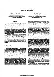
Fig. 8. (a) Test case 1. One of the unobserved blocks of data sz , i = 1; . . . ; 3, 300 pixels in size, extracted from the SPOT image shown in Fig. 6. 100 (b) Test case 1. HCM clustering of (a), with number of clusters L = 21, where cluster types are depicted by pseudocolors. (c) Test case 1. Four-adjacency neighboring edge map of (b).

2

results provided by, say, the standard resubstitution or holdout methods may not be in line with qualitative results by expert photointerpreters [29]. The proposed unsupervised DAMA strategy is employed to mitigate, with a mimimum of human intervention, the small and unrepresentative sample problem, which affects the estimation and comparison of image mapping systems in test cases 1 and 2. DAMA is implemented as follows. In test case 1, three nonover, , 100 lapping blocks of unobserved data 300 pixels in size, are extracted from Fig. 6 (in column-line coordinates, columns: 213 512, lines: 100 199, columns: 213 512, lines: which is shown in Fig. 8(a); columns: 1 300, lines: 413 512), ac240 339; cording to the RMC procedure (see Section V-A). In test case 2, which is less fragmented than test case 1, unobserved image


867

TABLE V TAXONOMY OF THE DATA LABELING ALGORITHMS ADOPTED FOR COMPARISON. LEGENDA: Y: YES, N: NO; P: PARAMETRIC. NP: NONPARAMETRIC

areas, which must be spectrally simple to analyze, can be larger than those in test case 1. Thus, two unobserved image areas ( ) 400 400 pixels in size, are extracted from the top left and bottom right corners of the raw image , respectively. According to the DAMA strategy, each unobserved block of data , , is clustered separately by a standard clustering algorithm to generate an implicit reference cluster map , . In our experiments, the standard HCM vector quantizer found in a commercial image processing software toolbox [2] is arbitrarily adopted in test case 1, whereas the enhanced Linde–Buzo–Gray (ELBG) vector quantizer [42], implemented in-house as a nearly optimal version of HCM (i.e., ELBG is nearly independent of random initialization), is arbitrarily employed in test case 2. These arbitrary selections are intended to stress the fact that DAMA is not required to exploit any specific clustering algorithm. With regard to the operational hypotheses implicitly made by DAMA at this stage, it is to be noted that, when employed for clustering, HCM-based vector quantizers are expected to perform well only with approximately equiprobable convex datasets [3] (refer to Section V-A, point 2). As an example of implicit reference cluster map made from , see Fig. 8(b). Let be the portion of map that overlaps with . According to the DAMA strategy (see Section V-B): 1) the labeling fidelity of the explicit submap to the reference cluster map is computed as the overall accuracy of the square, reshuffled overlapping area matrix OAMS , , , where OAMS in test case 1, and in test case 2; and 2) the spatial fidelity of results to reference data is computed as the mean absolute difference (in range [0, 4]) between the two four-adjacency edge maps extracted from maps and [as shown in Fig. 8(c)]. To summarize, DAMA provides two map quality indexes (namely, one labeling plus one spatial fidelity index), times three (respectively, two) cluster maps in test case 1 (respectively, test case 2), for each th competing classifier, . In combination with the unsupervised DAMA strategy, additional measures of classification success can be computed in badly posed image classification problems, such as test cases 1 and 2. Since ground truth ROIs are available and fully employed for training the inducer, a confusion matrix, computed between the output map and the available representative dataset, allows estimation of the so-called resubstitution error (upon the training dataset). If the resubstitution (learning) error is small, then bias is low, which means that the prior knowledge has been passed on to the image mapping system successfully. This is a

necessary condition to keep the combination of bias with variance low, but says nothing about the generalization capability of the image mapping system. A fourth feature that may be considered important in the assessment of competing classifiers is computation time, which affects the application domain of RS image mapping systems [29], [38]. However, since it is not directly related to the proposed DAMA strategy, computation time will be ignored in this experimental session. C. Set of Algorithms to Be Compared In the framework of the DAMA strategy for the quality assessment of competing maps, a comparison between image mapping systems is: 1) possible, whenever the (supervised) classifier or (unsupervised) clustering algorithm generates a (discrete, labeled) map and 2) fair, if the prior knowledge, having the initial form of ground truth ROIs, adapts its maximally informative representation to the learning strategies of the image mapping system at hand. Starting from these considerations, five well-known data labeling algorithms, featuring rather different architectural properties, are selected from the literature for comparison purposes. These algorithms are either nonparametric, like the context-insensitive (i.e., pixel-based) memory-based probabilistic neural network (PNN) classifier [48], or parametric, like the single-scale context-sensitive iterative conditional mode (ICM)-based maximum a posteriori (MAP)-Markov random field (MRF) classifier [49], the pixel-based plug-in nearest prototype (NP) (also called minimum-distance-to-mean [28], [50]) and Gaussian maximum-likelihood (ML) classifiers [3], both taken from a commercial image processing software toolbox [2], and the recently published pixel-based semisupervised expectation–maximization (SEM) classifier [7], which is capable of working in either supervised or unsupervised learning mode, identified with acronyms SEM1 and SEM2, respectively. A rough taxonomy of the compared data labeling algorithms is proposed in Table V. D. Initialization Strategies Before starting the learning sessions of competing inducers, prior knowledge, having the initial form of ground truth ROIs, must adapt its maximally informative representation to the learning properties of the system at hand (refer to Table V). In a parametric labeling algorithm (either supervised or unsupervised), the number of template vectors (also called reference vectors, prototypes, or codewords) is assumed coincident with the number of surface types of interest (in a classification

868


framework, these systems are known as one-prototype classifiers [50]). This implies that the distribution of class-specific representative samples is assumed to be consistent with the model of the class-specific spectral distributions adopted by the parametric labeling algorithm. In cases of adaptive iterative unsupervised SEM1, and supervised SEM2 and ICM-MAP-MRF, class-specific mean vectors are extracted from class-specific ROIs and passed on to an NP classification stage to extract initial estimates of image-wide class-specific (mean vector, covariance matrix) pairs. In the case of plug-in classifiers, like NP and ML, class-specific template vectors are extracted from ROIs by the external analyst and plugged into the classifier. These fixed template vectors are category-specific mean vectors in the case of NP, and category-specific (mean vector, covariance matrix) pairs in the case of ML. In cases of memory-based classifier PNN and iterative classifier SEM2, all representative labeled samples, belonging to ground truth ROIs, are passed on to the inducer to optimize the system’s free parameters during training.

Fig. 9. Test case 1. PNN classification map of the three-band SPOT image shown in pseudocolors (number of classes L = 21). To enhance human interpretability of mapping results, pseudocolors are chosen to mimic the true colors of surface classes (refer to footnote 6).

VII. EXPERIMENTAL RESULTS Class-conditional distributions in nonadaptive classifiers (either parametric, like NP and ML, or nonparametric, like PNN; see Section VI-C) are modeled on the basis of samples extracted from supervised ground truth ROIs exclusively, i.e., without considering unlabeled samples. Thus, NP, ML, and PNN are expected to perform well in minimizing the resubstitution error (where bias must be low). On the other hand, parametric iterative (adaptive) labeling algorithms (like ICM-MAP-MRF, SEM1, and SEM2), where all unlabeled samples contribute to the adaptation of category-specific template vectors, are expected to improve their generalization ability on unobserved image areas (when the combination of bias with variance must be kept low) at the cost of a possible increase in their resubstitution error on ground truth ROIs (due to an increase in bias). A. Test Case 1 This test image, depicting a urban scene with many small image segments featuring a homogeneous spectral response, is more fragmented than test case 2. The maximum number of iterations is set equal to 10 in iterative algorithms, namely, ICM-MAP-MRF, SEM1, and SEM2. With regard to the ICM-MAP-MRF algorithm, it is obvious that optimal, MRF-based smoothing parameters (two-point cliques) , , are both class- and application-dependent. To avoid a time-consuming, class-specific, trial-and-error parameter selection strategy that would represent a degree of user’s supervision superior to that required by the rest of the algorithms involved in our comparison, we set two-point clique , , potential parameters independent of the class. This choice is in line with recommendations found in [49], where is claimed to be independent of , because larger values of would the dataset if lead to excessive smoothing of regions. In PNN, spread parameter is set to 0.6 after a class-independent trial-and-error

Fig. 10. Test case 1. SEM2 classification map of the three-band SPOT image shown in pseudocolors (number of classes L = 21). To enhance human interpretability of mapping results, pseudocolors are chosen to mimic the true colors of surface classes (refer to footnote 6).

TABLE VI TEST CASE 1. RESUBSTITUTION OVERALL ACCURACY (SUM OF DIAGONAL ELEMENTS OF THE CONFUSION MATRIX) BETWEEN LABELING RESULTS AND REFERENCE DATA (ROIS) (BEST WHEN LARGEST). NUMBER OF LABEL TYPES (= number of ground truth ROIs) = 21. 3: WITHOUT SUPERVISED (TRAINING) SAMPLES. 33: WITH SUPERVISED (TRAINING) SAMPLES. RANK1 IS BEST WHEN SMALLEST

selection procedure, which is fast and easy, also due to the sensitivity of PNN to a small range of values.


869

TABLE VII TEST CASE 1. OVERLAPPING AREA (SUM OF DIAGONAL ELEMENTS OF THE CONFUSION MATRIX AFTER RESHUFFLING) BETWEEN THE EXPLICIT SUBMAP x AND THE IMPLICIT REFERENCE CLUSTER MAP x , i = 1; . . . ; 3 (BEST WHEN LARGEST). NUMBER OF LABEL TYPES (= number of ground truth ROIs) = 21. RANK2 IS BEST WHEN SMALLEST

TABLE VIII TEST CASE 1. MEAN AND STANDARD DEVIATION OF THE IMAGE COMPUTED AS THE ABSOLUTE DIFFERENCE BETWEEN THE TWO EDGE MAPS MADE FROM x AND x , i = 1, 2, 3 (BEST WHEN SMALLEST). RANK3 IS BEST WHEN SMALLEST

As two interesting examples of the mapping results obtained with this parameter setting, Figs. 9 and 10 show (in pseudocolors)6 the maps generated with, respectively, PNN and SEM2 classifiers (whose functional properties are quite different, refer to Table V) (the other output maps are omitted to save presentation space). According to perceptual quality criteria adopted by expert photointerpreters, SEM2 appears to perform better than PNN. In the framework of a resubstitution error estimation method, Table VI reports the training accuracy between labeling results and ground truth ROIs. Table VI shows that, in line with theoretical expectations, the resubstitution accuracy of SEM is largely inferior to that of traditional nonparametric (PNN) and parametric nonadaptive classifiers (e.g., NP). The supervised classifier SEM2, performs better than its unsupervised counterpart SEM1, in line with theoretical expectations. Although a low resubstitution error is a desirable property (meaning low bias), results provided by Table VI are counterintuitive for expert photointerpreters employing perceptual quality criteria (e.g., see Figs. 9 and 10), which justifies the exploitation of the noncon6Every class index is associated to a pseudocolor chosen to mimic the true color of that surface class (e.g., three shades of blue are adopted to depict labels belonging to classes sea water 1 to sea water 3, etc.), to enhance human interpretability of mapping results.

ventional DAMA strategy to assess the generalization capabilities of competing classifiers. Table VII shows the maximum sum (after reshuffling) of diagonal elements of the overlapping area matrix computed between the explicit submap , and the reference cluster map , , 100 (adopted as the ground truth image) 300 pixels in size, generated by the HCM vector quantizer. Table VII reveals that the labeling fidelity of the output map generated by SEM to implicit reference cluster maps is superior to that of the other labeling approaches, where nonadaptive classifiers, like NP and PNN, perform rather poorly, in line with theoretical expectations. Parametric, adaptive, context-sensitive ICM-MAP-MRF, by enforcing spatial continuity in pixel labeling, is incapable of preserving genuine but small image details. To investigate the spatial fidelity of the output map to implicit reference cluster maps, Table VIII reports the mean and standard deviation of the edge map difference computed between and , . the two edge maps extracted from Table VIII shows that SEM is superior to the other algorithms in preserving genuine but small image details, irrespective of their labeling. These spatial fidelity results are somehow in contrast with the labeling fidelity results shown in Table VII, although the Spearman correlation value between Rank2 and Rank3 is

870


Fig. 11. Test case 2. PNN classification map of the seven-band Landsat TM image shown in pseudocolors (number of classes L = 12). To enhance human interpretability of mapping results, pseudocolors are chosen to mimic the true colors of surface classes (refer to footnote 6). The masked portion of the image is in black.

0.8857 (revealing strong agreement; see Section V-B). Overall, these conclusions appear to be consistent with those of expert photointerpreters and in line with the theoretical expectations concerning the algorithms’ potential utilities.

Fig. 12. Test case 2. SEM2 classification map of the seven-band Landsat TM image shown in pseudocolors (number of classes L = 12). To enhance human interpretability of mapping results, pseudocolors are chosen to mimic the true colors of surface classes (refer to footnote 6). The masked portion of the image is in black. TABLE IX TEST CASE 2. RESUBSTITUTION OVERALL ACCURACY (SUM OF DIAGONAL ELEMENTS OF THE CONFUSION MATRIX) BETWEEN LABELING RESULTS AND REFERENCE DATA (ROIS) (BEST WHEN LARGEST). NUMBER OF LABEL TYPES (= number of ground truth ROIs) = 12. RANK4 IS BEST WHEN SMALLEST

B. Test Case 2 This test image, depicting an agricultural site, is less fragmented than test case 1. As a consequence, in this experiment, functional benefits deriving from using the single-scale, context-sensitive ICM-MAP-MRF algorithm, which is provided with an MRF-based mechanism to enforce spatial continuity in pixel labeling, are expected to be superior to those in test case 1. User-defined parameters are the same as those selected in test case 1, except for spread parameter in PNN, which is set equal to 1.0 after (an easy and fast) trial-and-error selection procedure. As in test case 1, interesting examples of the mapping results obtained with this parameter setting are shown in Figs. 11 and 12, where two maps generated with, respectively, classifier PNN and SEM2 are depicted (in pseudocolors). In test case 2, due to its large fragmentation and to the absence of easy-to-recognize built-up areas, it is very difficult for expert photointerpreters to determine whether, for example, PNN (see Fig. 11) performs better than SEM2 (see Fig. 12). In the framework of a resubstitution error estimation method, Table IX shows the overall accuracy (sum of diagonal elements of the confusion matrix) between output mapping results and ground truth ROIs. In this experiment, the nontraditional algorithm (SEM) is more competitive with traditional labeling approaches (like NP, ML, and PNN), than in test case 2 (refer to Table VI). Table X shows the maximum sum (after reshuffling) of the elements on the main diagonal of the overlapping area matrix computed between the reference cluster map (generated by , the ELBG vector quantizer) and the explicit submap , with . In Table X, SEM provides a labeling

fidelity of output results to multiple cluster maps superior to those of the other image labeling approaches, in line with test case 1 (refer to Table VII). To investigate the spatial fidelity of segmentation results to reference data, Table XI reports the mean and standard deviation of the difference edge map computed between the two edge and , with . In contrast with remaps made from sults shown in Table X, Table XI reveals that SEM is ranked average in preserving genuine but small image details, irrespective of their labeling. The Spearman correlation value between Rank5 and Rank6 is 0.4857 (revealing poor agreement; refer to Section V-B), which justifies the separate computation of labeling and spatial fidelity indexes for map quality assessment. Overall, these conclusions are consistent with those of test case 1 (see Section VII-A) and with theoretical expectations concerning the algorithms’ potential utilities. VIII. CONCLUSION The unsupervised DAMA strategy is proposed to quantitatively assess the (subjective) quality of thematic maps generated from RS images when little or no ground truth knowledge is available. The core of DAMA consists of a semiautomatic procedure where multiple reference cluster maps, independent of the available representative dataset (if any), are generated


871

TABLE X TEST CASE 2. OVERLAPPING AREA (SUM OF DIAGONAL ELEMENTS OF THE CONFUSION MATRIX AFTER RESHUFFLING) BETWEEN x AND x , i = 1; 2 (BEST WHEN LARGEST). NUMBER OF LABEL TYPES (= number of ground truth ROIs) = 12. RANK5 IS BEST WHEN SMALLEST

TABLE XI TEST CASE 2. MEAN AND STANDARD DEVIATION OF THE IMAGE COMPUTED AS THE ABSOLUTE DIFFERENCE BETWEEN MAPS MADE FROM x AND x , i = 1, 2 (BEST WHEN SMALLEST). RANK6 IS BEST WHEN SMALLEST

from blocks of unobserved data (called unlabeled candidate representative raw areas) with a minimum of human intervention. To assess the consistency between the map under investigation and multiple reference cluster maps, DAMA computes labeling as well as spatial quality indexes. This is a potential improvement over traditional map accuracy assessment techniques, where the spatial fidelity of maps to reference data is ignored in practice. Although intrinsically heuristic (due to the subjective nature of the clustering problem) and noninjective (like any evaluation measure), DAMA is expected to be particularly useful in poorly to ill-posed image classification comparative problems (i.e., in image classification applications affected by the small/unrepresentative sample problem), where the confidence in the estimated classification error rate (computed by traditional, heuristic supervised resampling techniques) is low (due to the small size of the test set). In this paper, DAMA is applied to two badly posed RS image classification problems in combination with the holdout resampling technique. This combination provides quantitative results that, in line with theoretical expectations and qualitative results by human photointerpreters, appear to be useful in estimating and comparing the generalization capabilities of competing induced classifiers in badly posed image mapping tasks. As a future development of this work, additional experiments will be planned where DAMA and the approach proposed in [44] are adopted in the estimation and comparison of standard discrete mapping systems applied to badly posed image classification tasks.

THE

TWO EDGE

ACKNOWLEDGMENT The authors wish to thank the Associate Editor and anonymous reviewers for their helpful comments. P. C. Smits, as a member of the GRSS-DFC, is acknowledged for providing the grss_dfc_0004 Landsat TM image. REFERENCES [1] R. G. Congalton and K. Green, Assessing the Accuracy of Remotely Sensed Data. Boca Raton, FL: Lewis, 1999. [2] ENVI User’s Guide, Research Systems Inc., Boulder, CO, 2003. [3] C. M. Bishop, Neural Networks for Pattern Recognition. Oxford, U.K.: Clarendon, 1995. [4] A. K. Jain, R. Duin, and J. Mao, “Statistical pattern recognition: a review,” IEEE Trans. Pattern Anal. Mach. Intell., vol. 22, no. 1, pp. 4–37, Jan. 2000. [5] G. G. Wilkinson, “Are remotely sensed image classification techniques improving? Results of a long term trend analysis,” presented at the IEEE Workshop on Advances in Techniques for Analysis of Remotely Sensed Data, Greenbelt, MD, Oct. 27–28, 2003. [6] M. P. Buchheim and T. M. Lillesand, “Semi-automated training field extraction and analysis for efficient digital image classification,” Photogramm. Eng. Remote Sens., vol. 55, no. 9, pp. 1347–1355, 1989. [7] Q. Jackson and D. Landgrebe, “An adaptive classifier design for highdimensional data analysis with a limited training data set,” IEEE Trans. Geosci. Remote Sensing, vol. 39, no. 12, pp. 2664–2679, Dec. 2001. [8] P. H. Swain and S. M. Davis, Remote Sensing: The Quantitative Approach. New York: McGraw-Hill, 1978. [9] E. Binaghi, I. Gallo, G. A. Lanzarone, and M. Pepe, “Remote sensing object recognition by cognitive pyramids,” in Geospatial Pattern Recognition, E. Binaghi, P. Brivio, and S. Serpico, Eds. Kerala, India: Research Signpost/Transworld Research, Apr. 2002, pp. 87–103. [10] G. M. Foody, “Approaches for the production and evaluation of fuzzy land cover classifications from remotely-sensed data,” Int. J. Remote Sens., vol. 17, pp. 1317–1340, 1996.

872


[11] V. Cherkassky and F. Mulier, Learning From Data: Concepts, Theory, and Methods. New York: Wiley, 1998. [12] R. Xu and D. Wunsch, II, “Survey of clustering algorithms,” IEEE Trans. Neural Netw., 2005, to be published. [13] R. Kohavi, “A study of cross-validation and bootstrap for accuracy estimation and model selection,” presented at the Int. Joint Conf. Artificial Intelligence, 1995. [14] R. Kothari and V. Jain, “Learning from labeled and unlabeled data using a minimal number of queries,” IEEE Trans. Neural Netw., vol. 14, no. 6, pp. 1496–1505, Nov. 2003. [15] G. M. Foody, “Status of land cover classification accuracy assessment,” Remote Sens. Environ., vol. 80, pp. 185–201, 2002. [16] M. M. Durat and D. A. Landgrebe, “A cost-effective semisupervised classifier approach with kernels,” IEEE Trans. Geosci. Remote Sens., vol. 42, no. 1, pp. 264–270, Jan. 2004. [17] A. Baraldi and E. Alpaydin, “Constructive feedforward ART clustering networks—Part I,” IEEE Trans. Neural Netw., vol. 13, no. 3, pp. 645–661, May 2002. , “Constructive feedforward ART clustering networks—Part II,” [18] IEEE Trans. Neural Netw., vol. 13, no. 3, pp. 662–677, May 2002. [19] B. Fritzke. (1997) Some competitive learning methods. [Online]. Available: http://www.ki.inf.tu-dresden.de/~fritzke/JavaPaper. [20] E. Backer and A. K. Jain, “A clustering performance measure based on fuzzy set decomposition,” IEEE Trans. Pattern Anal. Mach. Intell., vol. PAMI-3, no. 1, pp. 66–75, Jan. 1981. [21] R. O. Duda, P. E. Hart, and D. G. Stork, Pattern Classification, 2nd ed. New York: Wiley, 2001. [22] M. R. Spiegel, Statistics. New York: McGraw-Hill, 1961. [23] G. Buttner, T. Hajos, and M. Korandi, “Improvements to the effectiveness of supervised training procedures,” Int. J. Remote Sens., vol. 10, no. 6, pp. 1005–1013, 1989. [24] B. Efron, The Jackknife, the Bootstrap and Other Resampling Plans. Philadelphia, PA: SIAM, 1982. [25] J. T. Morgan, A. Henneguelle, J. Ham, J. Ghosh, and M. M. Crawford, “Adaptive feature spaces for land cover classification with limited ground truth,” Int. J. Pattern Recognit. Artif. Intell., vol. 18, no. 5, pp. 777–799, 2004. [26] S. B. Serpico and L. Bruzzone, “A new search algorithm for feature selection in hyperspectral remote sensing images,” IEEE Trans. Geosci. Remote Sens., vol. 39, no. 7, pp. 1360–1367, Jul. 2001. [27] L. Bruzzone and S. Serpico, “An iterative technique for the detection of land cover transitions in multitemporal remote sensing images,” IEEE Trans. Geosci. Remote Sens., vol. 35, no. 4, pp. 858–867, Jul. 1997. [28] T. Lillesand and R. Kiefer, Remote Sensing and Image Interpretation, 3rd ed. New York: Wiley, 1994. [29] A. Baraldi, M. Sgrenzaroli, and P. Smits, “Contextual clustering with label backtracking in remotely sensed image applications,” in Geospatial Pattern Recognition, E. Binaghi, P. Brivio, and S. Serpico, Eds. Kerala, India: Research Signpost/Transworld Research, Apr. 2002, pp. 117–145. [30] M. Beauchemin and K. Thomson, “The evaluation of segmentation results and the overlapping area matrix,” Int. J. Remote Sens., vol. 18, no. 18, pp. 3895–3899, 1997. [31] L. Bruzzone, “An approach to feature selection and classification of remote-sensing images based on the Bayes rule for minimum cost,” IEEE Trans. Geosci. Remote Sens., vol. 38, no. 1, pp. 429–438, Jan. 2000. [32] P. Smits, S. Dellepiane, and S. Schowengerdt, “Quality assessment of image classification algorithms for land cover mapping: A review and proposal for a cost-based approach,” Int. J. Remote Sens., vol. 20, pp. 1461–1486, 1999. [33] R. Haralick and L. Shapiro, “Survey of image segmentation techniques,” Comput. Vis., Graphics, Image Process., vol. 29, pp. 100–132, 1985. [34] J. Liu and Y. Yang, “Multiresolution color image segmentation,” IEEE Trans. Pattern Anal. Mach. Intell., vol. 16, no. 7, pp. 689–700, Jul. 1994. [35] M. Heath, S. Sarkar, T. Sanocki, and K. Bowyer, “Comparison of edge detectors: a methodology and initial study,” in Computer Vision and Pattern Recognition ’96, San Francisco, CA, Jun. 1996. [36] A. Hoover, G. Jean-Baptiste, X. Jiang, P. Flynn, H. Bunke, D. Goldgof, K. Bowyer, D. Eggert, A. Fitzgibbon, and R. Fisher, “An experimental comparison of range image segmentation algorithms,” IEEE Trans. Pattern Anal. Machine Intelligence, vol. 18, no. 7, pp. 673–688, Jul. 1996.

[37] L. Delves, R. Wilkinson, C. Oliver, and R. White, “Comparing the performance of SAR image segmentation algorithms,” Int. J. Remote Sens., vol. 13, no. 11, pp. 2121–2149, 1992. [38] M. Sgrenzaroli, A. Baraldi, H. Eva, G. De Grandi, and F. Achard, “Contextual clustering for image labeling: An application to degraded forest assessment in Landsat TM images of the Brazilian Amazon,” IEEE Trans. Geosci. Remote Sens., vol. 40, no. 8, pp. 1833–1847, Aug. 2002. [39] G. M. Foody, “Thematic mapping from remotely sensed data with neural networks: MLP, RBF and PNN based approaches,” J. Geograph. Syst., vol. 3, pp. 217–232, 2001. [40] S. Serpico, L. Bruzzone, and F. Roli, “An experimental comparison of neural and statistical nonparametric algorithms for supervised classification of remote-sensing images,” Pattern Recognit. Lett., vol. 17, no. 13, pp. 1331–1341, 1996. [41] L. Bruzzone and D. F. Prieto, “A technique for the selection of kernelfunction parameters in RBF neural networks for classification of remotesensing images,” IEEE Trans. Geosci. Remote Sens., vol. 37, no. 2, pp. 1179–1184, Mar. 1999. [42] G. Patanè and M. Russo, “The enhanced-LBG algorithm,” Neural Netw., vol. 14, no. 9, pp. 1219–1237, 2001. [43] A. Baraldi, P. Blonda, F. Parmiggiani, and G. Satalino, “Contextual clustering for image segmentation,” Opt. Eng., vol. 39, no. 4, pp. 1–17, Apr. 2000. [44] J. T. Finn, “Use of the average mutual information index in evaluating classification error and consistency,” Int. J. Geograph. Inf. Syst., vol. 7, no. 4, pp. 349–366, 1993. [45] L. Prechelt, “A quantitative study of experimental evaluations of neural network learning algorithms: Current research practice,” Neural Netw., vol. 9, no. 3, pp. 457–462, 1996. [46] P. Lukowicz, E. Heinz, L. Prechelt, and W. Tichy, “Experimental evaluation in computer science: A quantitative study,” Univ. Karlsruhe, Karlsruhe, Germany, Tech. Rep. 17/94, 1994. [47] T. Mitchell, Machine Learning. New York: McGraw-Hill, 1997. [48] D. Specht, “Probabilistic neural networks,” Neural Netw., vol. 3, pp. 109–118, 1990. [49] E. Rignot and R. Chellappa, “Segmentation of polarimetric synthetic aperture radar data,” IEEE Trans. Image Process., vol. 1, no. 3, pp. 281–300, Jul. 1992. [50] J. C. Bezdek, T. R. Reichherzer, G. S. Lim, and Y. Attikiouzel, “Multiple-prototype classifier design,” IEEE Trans. Syst., Man, Cybern., C, vol. 28, no. 1, pp. 67–79, Feb. 1998. [51] R. Lunetta and D. Elvidge, Remote Sensing Change Detection: Environmental Monitoring Methods and Applications. London, U.K.: Taylor & Francis, 1999.

Andrea Baraldi was born in Modena, Italy, in 1963. He received the laurea degree in electronic engineering from the University of Bologna, Bologna, Italy, in 1989. His master’s thesis focused on the development of unsupervised clustering algorithms for optical satellite imagery. He is currently a Research Associate with the Institute of Intelligent Systems for Automation, National Research Council (ISSIA-CNR), Bari, Italy. From 1989 to 1990, he was a Research Associate at CIOC-CNR, an Institute of the National Research Council, Bologna, and served in the army at the Istituto Geografico Militare in Florence, working on satellite image classifiers and GIS. As a consultant at ESA-ESRIN, Frascati, Italy, he worked on object-oriented applications for GIS from 1991 to 1993. From December 1997 to June 1999, he joined the International Computer Science Institute, Berkeley, CA, with a postdoctoral fellowship in artificial intelligence. From 2000 to 2002, he was a Post-Doc Researcher with the European Commission Joint Research Center, Ispra, Italy, where he worked on the development and validation of algorithms for the automatic thematic information extraction from wide-area radar maps of forest ecosystems. Since his master thesis, he has had continual interaction with ISAC-CNR, Bologna. His main interests center on image segmentation and classification, with special emphasis on texture analysis and neural network applications employing contextual image information. Dr. Baraldi is an Associate Editor of IEEE TRANSACTIONS ON NEURAL NETWORKS.


Lorenzo Bruzzone (S’95–M’99–SM’03) received the laurea (M.S.) degree in electronic engineering (summa cum laude) and the Ph.D. degree in telecommunications, both from the University of Genoa, Genoa, Italy, in 1993 and 1998, respectively. He is currently Head of the Remote Sensing Laboratory in the Department of Information and Communication Technologies at the University of Trento, Trento, Italy. From 1998 to 2000, he was a Postdoctoral Researcher at the University of Genoa. From 2000 to 2001, he was an Assistant Professor at the University of Trento, where he has been an Associate Professor of telecommunications since November 2001. He currently teaches remote sensing, advanced pattern recognition, and electrical communications. His current research interests are in the area of remote sensing image processing and recognition (analysis of multitemporal data, feature selection, classification, data fusion, and neural networks). He conducts and supervises research on these topics within the frameworks of several national and international projects. He is the author (or coauthor) of more than 110 scientific publications, including journals, book chapters, and conference proceedings. He is a referee for many international journals and has served on the Scientific Committees of several international conferences. Dr. Bruzzone ranked first place in the Student Prize Paper Competition of the 1998 IEEE International Geoscience and Remote Sensing Symposium (Seattle, July 1998). He is the Delegate in the scientific board for the University of Trento of the Italian Consortium for Telecommunications (CNIT) and a member of the Scientific Committee of the India–Italy Center for Advanced Research. He was a recipient of the Recognition of IEEE Transactions on Geoscience and Remote Sensing Best Reviewers in 1999 and was a Guest Editor of a Special Issue of the IEEE TRANSACTIONS ON GEOSCIENCE AND REMOTE SENSING on the subject of the analysis of multitemporal remote sensing images (November 2003). He was the Chair and Co-chair of, respectively, the First and Second IEEE International Workshop on the Analysis of Multi-temporal Remote-Sensing Images (Trento, Italy, September 2001—Ispra, Italy, July 2003). Since 2003, he has been the Chair of the SPIE Conference on Image and Signal Processing for Remote Sensing (Barcelona, Spain, September 2003—Maspalomas, Gran Canaria, September 2004). He is an Associate Editor of the IEEE GEOSCIENCE AND REMOTE SENSING LETTERS. He is a member of the International Association for Pattern Recognition (IAPR) and of the Italian Association for Remote Sensing (AIT).

873

Palma Blonda (M’93) received the Ph.D. degree in physics from the University of Bari, Bari, Italy, in 1980. In 1984, she joined the Institute for Signal and Image Processing (now the Institute of Intelligent Systems for Automation), Italian National Research Council (ISSIA-CNR), Bari. Her research interests include digital image processing, fuzzy logic and neural networks, and soft computing applied to the integration and classification of multisource remote sensed data. She has recently been involved with the Landslide Early Warning Integrated System (LEWIS) Project, founded by the European Comunity in the framework of Fifth PQ. In this project, her research activity focuses on the application of multisource data integration and classification techniques for the extraction of EO-detectable superficial changes of some landslide-related factors to be used in early-warning mapping.

Quality Assessment of Classification and Cluster Maps ... - IEEE Xplore

Quality Assessment of Classification and Cluster Maps ... - IEEE Xplore

Suggest Documents

Automatic Quality Assessment of Echocardiograms ... - IEEE Xplore

Texture Classification - IEEE Xplore

Power quality detection and classification using wavelet ... - IEEE Xplore

Classification, Domains and Risk Assessment in Asset ... - IEEE Xplore

Radiometric, Geometric, and Image Quality Assessment ... - IEEE Xplore

Automatic Cluster Parallelization and Minimizing ... - IEEE Xplore

Risk Assessment - IEEE Xplore

Quality of Adaptation - IEEE Xplore

Comparative Assessment of Sleep Quality Estimates ... - IEEE Xplore

Nonintrusive Quality Assessment of Noise Suppressed ... - IEEE Xplore

Survey on Assessment of Power Quality Cost in ... - IEEE Xplore

Blind Image Quality Assessment Using Joint Statistics of ... - IEEE Xplore

Quality Assessment of Despeckled SAR Images - IEEE Xplore

Characterizing Location and Classification Error ... - IEEE Xplore

RADAR TARGET TYPE CLASSIFICATION AND ... - IEEE Xplore

Vehicle Segmentation and Classification Using ... - IEEE Xplore

Heterogeneous Domain Adaptation and Classification ... - IEEE Xplore

Assessment of Communication Technologies and ... - IEEE Xplore

IEEE AWPL Special Cluster on Wireless Power and ... - IEEE Xplore

Cryptosystems with discretized chaotic maps - IEEE Xplore

TEMPORAL FILTERING FOR DEPTH MAPS ... - IEEE Xplore

Estimating Pharmacokinetic Parameter Maps from ... - IEEE Xplore

SPATIO-TEMPORAL CONSISTENT DEPTH MAPS ... - IEEE Xplore

Automatic Modulation Classification of Overlapped ... - IEEE Xplore