c World Scienti c Publishing Company. CLUSTER VS ..... 2-D Ising model, however, the \world record" size in 3-D is L 3072, 14 hence the cross-over size for the ...
International Journal of Modern Physics C
c World Scienti c Publishing Company
CLUSTER VS SINGLE-SPIN ALGORITHMS { WHICH ARE MORE EFFICIENT? N. Itoy and G.A. Kohring
HLRZ at the KFA Julich Postfach 1913, D-5170 Julich, Germany y and Computing and Information Systems Center Japan Atomic Energy Research Institute Tokai, Ibaraki 319-11, Japan
Received Revised
(to be inserted by Publisher)
ABSTRACT A comparison between single-cluster and single-spin algorithms is made for the Ising model in 2 and 3 dimensions. We compare the amount of computer time needed to achieve a given level of statistical accuracy, rather than the speed in terms of site updates per second or the dynamical critical exponents. Our main result is that the cluster algorithms become more e�cient when the system size, Ld , exceeds, L � 70{300 for d = 2 and L � 80{200 for d = 3. The exact value of the crossover is dependent upon the computer being used. The lower end of the crossover range is typical of workstations while the higher end is typical of vector computers. Hence, even for workstations, the system sizes needed for e�cient use of the cluster algorithm is relatively large. Keywords : cluster algorithms, Ising models, vectorization, critical slowing down
1. Introduction The phenomena of critical slowing down within computer simulations of statistical systems near a second-order phase transition has been known for many years. The basic problem stems from the di�culty encountered by the traditional Metropolis Monte Carlo method of ipping individual spins when the correlation length is very large. In such a case, any given spin will tend to allign itself with those spins with which it is correlated, thus the problem of ipping a given spin becomes the problem of ipping the cluster of spins correlated with the given spin. This latter task can be quite time consuming when using a single-spin ip algorithm, because only small parts of a cluster are likely to be ipped during a single pass through the lattice. Obviously, it would be better to have an algorithm which can ip the entire cluster of correlated spins during a single pass through the lattice. A suitable de nition for a cluster of correlated spins was rst given by Fortuin
and Kasteleyn.1 Coniglio and Klein later showed that there is a correspondence between the Fortuin and Kasteleyn clusters and Fisher's droplet ideas.2 In 1983, Sweeny3 rst applied these ideas directly to the problem of critical slowing down in the Ising model. However, Sweeny's approach was di�cult to realize in practice and was never widely used. In 1987, Swendsen and Wang 4 presented an alternative approach which was easier to implement and to generalize to systems other than the Ising model. In the Swendsen-Wang procedure, all possible Fortuin-Kastelyn clusters are identi ed and then each is ipped with probability 1/2. Following Swendsen and Wang several authors proposed that equivilent results could be achieved by simply identifying and ipping a single cluster chosen at random.5 Since only that cluster which is to be ipped needs to be identi ed, this method should be faster and simpler than the Swendsen-Wang approach. In the literature there have been many claims about the e�ciency of the cluster methods vis-�a-vis the traditional single-spin ip algorithms.6 Most of these claims rest upon the calculation of the autocorrelation exponent z , which determines the asymptotic e�ciency of the algorithm for very large systems. However, while the cluster methods were developing the traditional Metropolis Monte Carlo algorithms were also moving forward through the development of sophisticated vectorized algorithms.7 9 Today, the typical time needed to update a single spin with a vector machine is on the order of a nanosecond. A more relevant question, then, is the amount of cpu time needed to obtain a given statistical accuracy for system sizes of practical importance. Here, we examine this question for both vector computers and scalar workstations. Our main result being, that even for scalar workstations, the system sizes where the cluster methods become more e�cient are relatively large.
2. The algorithms
The spin models we wish to use for our comparisons are the simple Ising models in two and three dimension. These models consist of of N spins, Si , arranged on a simple cubic lattice (Ld = N ) in d dimensions and taking on the values, f�1g. The spins interact only with their nearest neighbors. The traditional single-spin- ip Metropolis Monte Carlo method, proceeds as follows: 1) pick a spin, Si , either randomly or systematically; 2) calculate the change in energy, �E , which would occur if the spin were
ipped to its opposite value; 3) if �E < 0 then the spin ip is accepted otherwise the spin ip is accepted with probability exp ( � �E ), where is the inverse temperature of the system. Since each of the Si take on only two values, memory space can be saved by packing more than one variable into a computer word, the so-called multi-spin coding technique.7 The early practitioners of this technique worked with a single lattice, however it was latter realized that the updating speed could be greatly enhanced
by simulating multiple lattices. 8;9 Basically, the idea is to simulate B lattices simultaneously, on a computer with B bits per word. Originally, the multiple lattice technique was limited to simulating B di�erent temperatures as well, however, this restriction has also been lifted. 8 For the 3-D Ising model, these techniques currently enable one to reach speeds of nearly 466 million site updates per second (466 Mups) on a single Cray-YMP processor, 1040 Mups on the JAERI and NEC's experimental MONTE-4 machine and 2190 Mups on Fujitsu VP2600/10. The MONTE-4 is designed and constructed based on the NEC SX3/41 with some additional vector pipelines, and other improvements including a 2.5 nsec clock cycle.16 The reader interested in the details of this algorithm can nd them in ref. 9, while an example implementation is given in Appendix B. For the cluster- ip algorithms, one proceeds quite di�erently from the procedure given above. As stated in the introduction, one must identify a cluster of correlated spins and attempt to ip the entire cluster. The single cluster algorithm 5 works as follows: 1) pick a spin, Si , at random as the rst spin in the cluster; 2) if the neighboring spins are of the same sign as spin Si , then add them to the cluster with probability 1 e 2 , otherwise ignore them; 3) repeat 2) with the newly added spins until no new spins are added to the cluster; 4) ip all the spins in the cluster to their opposite value. As mentioned in the introduction, this single cluster algorithm is easier to implement than the full cluster algorithm because there is no need to label all of the individual clusters. This procedure is more complicated than the single-spin algorithm, hence the updating speeds of are generally quite small, approximately 0.1 Mups. Recently, it was shown, that the single cluster algorithm could be vectorized by vectorizing the cluster search over the active sites on the perimeter of the cluster.10 The kernel of such a vectorized algorithm is given in Appendix C. Obviously, this algorithm will only be e�cient if the vector length is \long enough". (Where the meaning of \long enough" is hardware dependent.) Fig. 1 shows a histogram of the vector length taken from a 2-D system with L = 512. The histogram is over 10,000 clusters taken at the critical temperature of the 2-D Ising model. In this example, the average vector length is 98, however, the most probable vector length is 19. This re ects the fact, that initially the cluster is quite small, hence there are very few points on the perimeter. As the cluster grows, so does the number of perimeter sites, however, at some point, the number of active sites on the perimeter reaches a maximum and then decreases until the cluster nally stops growing. Given, the wide distribution of vector lengths, the e�ciency of this algorithm on a vector computer depends upon how well the compiler handles short vector loops and how well the hardware and software can handle random memory accesses. In the next section, we test the e�ciency of this algorithm using vector and scalar computers.
0.008 L=512 0.007 0.006 0.005 0.004 0.003 0.002 0.001 0 0
100
200
300 400 vector length
500
600
Fig. 1. Histogram of the vector length for a 2-D system with L = 512. The histogram was made at the critical point using 10,000 clusters.
3. Results A comparison of the forementioned single-spin- ip and cluster- ip algorithms was made on vector and scalar computers. For the vector computers we chose the Cray-YMP/832 and the MONTE-4 two machines with very di�erent hardware characteristics and for the scalar machines we chose the SUN Sparc workstation series. When comparing the above algorithms, speed is not the only criterion, because the auto-correlation times are very di�erent. The auto-correlation time, � , measures the statistical accuracy achievable with n Monte Carlo p sweeps through the lattice. Typically, the statistical error, �, is given by: � � �= (n=� ), where � is the standard deviation in some measured quantity. At the critical temperature, Tc , it is known that for the above algorithms, � � Lz . Where zss � 2:0, for the single-spin case,11;12. For the single-cluster algorithm, it is customary to multiply the correlation time in terms of cluster ips by the average relative cluster size. In this way, one obtains the correlation time per spin ip, which has a z value of, zsc � 0:25.6 This practice is unfortunate, because one can only measure observables after each cluster has been ipped and not when a part of the cluster has been ipped, hence, to determine the required cpu resources, one must use the correlation time in terms of cluster ips. This correlation time is much larger than the one usually mentioned
in the literature6 , because the average relative cluster size tends to decrease like O(L2 d � ). Consequently, the e�ective z value for the cluster updating is given by: zeff = zsc + d + � 2. In 2-D, � = 0:25, which gives zeff = 0:50 for the single-cluster algorithm. Given the large speed di�erential and the large di�erence in z , the only reasonable criterion for comparing these two algorithms is by comparing the amount of cpu time needed to obtain a given level of statistical accuracy. Asymptotically, this cpu d+zss and tsc / Ld+zeff . Hence, asymptotically, the cluster time, tcpu , is tss cpu cpu / L algorithm will be more e�cient (i.e., require less cpu time) than the single-spin algorithm, however, the proportionality constants di�er considerably, because the cluster algorithm is more complex than the single-spin algorithm, so that for small systems the single-spin algorithms will be more e�cient. The question we want to ask here, is whether or not the system size at which the cross-over from single-spin e�ciency to cluster e�ciency is \reasonable". When calculating � there is one subtlety to be taken into account: di�erent observables can have di�erent values of � . In particular, even quantities like the energy and the susceptibility are expected to have � 's which are much di�erent than odd quantities like the magnetization, although most people expect that z should be independent of the observable in question. If the sampling interval of the quantity to be calculated, n in terms of Monte Carlo steps, is much large than � , then the the auto-correlation time for all even quantities, should be the same. However, when using the integrated correlation time, �int, as a measure of � , di�erent observables can strongly couple to one or more fast modes, thus under estimating the true value of � . In the 2-D case, we nd that estimates of �int for the energy converge to that of the magnetization squared, when measurements are done for n >> �int. For shorter runs, we observe a much smaller � for the energy than for the magnetization squared, hence, our comparisons here are made with �int as estimated for the magnetization squared. In the 3-D case, we nd a much smaller di�erence between the estimates of � taken from the magnetization squared and the energy even for rather short runs. In Fig. 2a is a plot of the cpu time necessary for 100 � �int measurements for the 2-D Ising model using single-spin and cluster algorithms on vector computers. (The raw data for all graphs is given in Appendix A.) For the single-spin algorithms we measure the speed in terms of Mups and then multiply this speed by the lattice size and 100 times the correlation time.11;12 For the cluster algorithm, we measure the average time needed to perform 100 cluster updates, then multiply this by the correlation time in terms of Monte-Carlo sweeps. We used the energy auto-correlation time as measured with the technique recently introduced in ref. 12. In all cases, the energy auto-correlation time per spin and its corresponding critical exponent are in agreement with results previously reported.6 The single-spin algorithm runs at a peak speed of 1290 Mups on the MONTE-4 and 720 Mups on the Cray-YMP (All times are for a single processor.). This speed di�erence re ects the di�erence in the clock cycle between the two machines. However, the peak speed of the cluster
10000 2D Vector Processor
1000
100
cpu second
10
1
0.1
Cray SS C MONTE-4 SS
0.01
C 0.001
0.0001 10
100
1000 L
Fig. 2a. Cpu time need to make 100 � �int time steps with the 2-D Ising model using the Cray-YMP and the MONTE-4 vector computers.
10000 2D Scalar Processor 1000
cpu second
100
10
Sparc 10 SS C
1
0.1
0.01
0.001 10
100 L
Fig. 2b. Same as (a) but for the SUN Sparc-10 scalar workstation.
10000
1000
3D Vector Processor
100
cpu second
10
1
0.1
Cray SS C MONTE-4 SS
0.01
C 0.001
0.0001 10
100 L
Fig. 3a. Cpu time need to make 100 � �int time steps with the 3-D Ising model using the Cray-YMP and the MONTE-4 vector computers.
100000 3D Scalar Processor 10000
cpu second
1000
100
10
1
Sparc 10 SS C
0.1
0.01 10
100 L
Fig. 3b. Same as (a) but for the SUN Sparc-10 scalar workstation.
updating is approximately the same for each machine, 1.0 Mups. This re ects the fact that the MONTE-4 machine performs very poorly for short vector loops, the most probable situation for the cluster algorithm. For the smallest system sizes, the Cray-YMP is running at a speed of only 21 million operations per second, while for the largest system sizes this speed increases to over 150 million operations per second, or about 60% of the YMP's sustainable speed. Hence, the vectorized cluster algorithms are indeed running e�ciently on vector machines. From g. 2a it can be seen that the cross-over size ranges from L � 200 for the Cray-YMP to L � 300 for the MONTE-4. Fig. 2b shows the results for the SUNSparc-10 workstation. For the SUN-Sparc-10 the cross-over size is L � 70. Hence, even on scalar workstations, the multi-spin coding algorithms are very e�cient, and contrary to common belief, the cross-over sizes are nearly the same as for the vector computers. These cross-over sizes are certainly small compared to the \world record" size of L = 169; 984,14 however, this world record size was only used to calculate the decay of the initial magnetization during the rst 100 time steps and was not used for measuring equilibrium properties, which is the primary purpose of Monte Carlo methods. On the other hand, since most of the equilibrium properties of the 2-D Ising Model can be calculated analytically, it is more interesting to look at the behavior of the above algorithms for the 3-D situation, where the equilibrium properties cannot be calculated exactly . Fig. 3a. shows the results for the 3-D Ising model on the vector computers. For the inverse critical temperature, c we use the estimate: c = 0:221656. Here we see that the cross-over sizes are L � 120 for the Cray-YMP and L � 200 for the MONTE-4. Fig. 3b gives the results for the SUN-Sparc-10 workstations. Here the cross-over size is about L � 80. These sizes are somewhat smaller than for the 2-D Ising model, however, the \world record" size in 3-D is L � 3072, 14 hence the cross-over size for the 3-D systems are relatively larger than for the 2-D systems. We can answer the question if these sizes are reasonable by looking at the high resolution studies of the 3-D Ising model performed by various groups in ref. 15. These papers have helped to set the current standard for accuracy in equilibrium Monte Carlo simulations. All three papers studied system sizes in the range 8 � L � 128. The rst two papers used single-spin ip algorithms, while the third paper used a single cluster algorithm. All three papers used roughly the same amount of computer resources and achieved nearly the same accuracy although they each analysed their data using di�erent methods. Hence, these papers support the results found here, namely for systems up to L � 100 200, there is no clear advantage to be gained by cluster updating. Larger systems would not have helped these researchers much because they simply did not have enough computer time at their disposal to study larger systems. Thus, as far as calculating thermodynamic properties is concerned, the sizes at which the cluster algorithms are clearly more e�cient than single-spin algorithms for the 3-D Ising model, are slightly larger than realistic, given the currently available computers and the currently known algorithms. This
situation may change, given faster scalar processors or parallel computers. However, since most of the announced parallel computers include vector co-processors, the cross-over size may also increase with increasing speed of the vector co-processors. Finally, it should be noted that single-spin algorithms have had a much longer time to develop than cluster-algorithms. Evertz's vectorized cluster algorithm is one step towards faster cluster algorithms and there is still hope for yet faster methods.
Acknowledgements
We would like to thank H.G. Evertz and D. Stau�er for many help discussions related to this work.
References 1. P.W. Kasteleyn and C.M. Fortuin, J. Phys. Soc. Jpn. Suppl. 26s (1969) 11. C.M. Fortuin and P.W. Kasteleyn, Physica 57 (1972) 536. 2. A. Coniglio and W. Klein, J. Phys. A. 13 (1980) 2775. 3. M. Sweeny Phys. Rev. B. 27 (1983) 4445. 4. R.H. Swendsen and J.-S. Wang, Phys. Rev. Lett. 58 (1987) 86. 5. U. Wol�, Phys. Rev. Lett. 62 (1989) 361. M. Hasenbusch, Nuclear Phys. B333 (1990) 581. 6. U. Wol�, Phys. Lett. B 228 (1989) 379. C.F. Baillie, Int. J. Mod. Phys. C 1 (1990) 91. J.-S. Wang and R.H. Swendsen, Physica A 167 (1990) 565. 7. R. Friedberg and J. Cameron, J. Chem. Phys. 52 (1970) 6049. R. Zorn, H.J. Herrmann and C. Rebbi, Comp. Phys. Comm. 23 (1981) 337. S. Wansleben, Comp. Phys. Comm. 43 (1987) 315. P.M.C. de Oliveira, Computing Boolean Statistical Models, (World Scienti c, Singapore, 1991). G. Bhanot, D. Duke and R. Salvador, J. Stat. Phys. 44 (1986) 985. 8. C. Michael, Phys. Rev. B 33 (1986) 7861. N. Ito, M. Kikuchi and Y. Okabe, Int. J. Mod. Phys. C. (to be published). 9. N. Ito and Y. Kanada, Supercomputer 5 (1988) 31; Supercomputer 7 (1990) 29; in Proc. of Supercomputing '90, (IEEE Computer Society Press, 1990) pp. 753-763. 10. H.G. Evertz, J. Stat. Phys. 70 (1993) 1075. 11. N. Ito, Physica A 192 (1993) 604; Phsica A (1993) (in press). 12. M. Kikuchi and N. Ito (in preparation). 13. J.G. Zabolitzky and H.J. Herrmann, J. Comp. Phys. 76 (1988) 426. 14. C. Munkel, D. Heermann, J. Adler, M. Gofman and D. Stau�er, Phsica A 193 (1993) 540. 15. A.M. Ferrenberg and D.P. Landau, Phys. Rev. B 44 (1991) 5081. N. Ito and M. Suzuki, J. Phys. Soc. Jpn. 60 (1991) 1978. N. Ito, in AIP Conf. Proc. 248, ed. C.K. Hu (AIP, 1992) pp. 136{142. C.F. Baillie, R. Gupta, K.A. Hawick and G.S. Pawley, Phys. Rev. B 45 (1992) 10438. 16. K. Asai, K. Higuchi, M. Akimoto, H. Matsumoto and Y. Seo in Proceedings of Mathematical Methods and Supercomputing in Nuclear Applications (Karlsruhe, 1993).
Appendix A Table 1: Single-Spin-Flip Measurements of the 2-D Ising Model. The necessary CPU time for 100� Monte Carlo steps is given in seconds. The gures in "large L" row refer to the prefactor of L4 16 (sec). int
:
size
CRAY YMP MONTE-4 Sparc 0.00098 0.00066 0.012 0.0035 0.0017 0.13 0.010 0.0050 0.62 0.053 0.027 4.6 0.18 0.097 19 0.75 0.39 79 11 6.5 1455 25 14 3304 2:8 � 10 9 1:6 � 10 9 3:6 � 10
�int
11 � 12 5:104 21 � 22 16:412 31 � 32 35:439 51 � 52 97:49 71 � 72 203:8 101 � 102 422:9 201 � 202 1931 301 � 302 4370 large L 0:020L2 16 :
7
S2 S10 0.0077 0.0053 0.085 0.063 0.39 0.27 2.9 2.0 12 3.8 50 38 906 572 2061 1286 2:3 � 10 7 1:4 � 10 7
Table 2: Single-Spin-Flip Measurements of the 3-D Ising Model. The necessary CPU time for 100� Monte Carlo steps is given in seconds. The gures in "large L" row refer to the prefactor of L5 03 (sec). int
:
size
�int
11 � 11 � 12 9.461 21 � 21 � 22 32.979 31 � 31 � 32 72.13 41 � 41 � 42 122.3 51 � 51 � 52 191.2 61 � 61 � 62 274.0 91 � 91 � 92 683 large L 0:065L2 03 :
CRAY YMP MONTE-4 Sparc 0.0044 0.0021 0.33 0.081 0.034 7.9 0.50 0.22 56 1.7 0.80 201 5.5 2.6 660 14 6.1 1625 100 50 14025 1:4 � 10 8 6:3 � 10 9 1:7 � 10
6
S2 0.20 4.9 34 124 408 1015 8447 1:0 � 10
6
S10 0.17 4.0 28 101 332 811 6749 8:2 � 10
Table 3: Single-Cluster-Flip Measurements of the 2-D Ising Model. The necessary CPU time for 100� Monte Carlo steps is given in seconds. E
size � < c > =L CRAY YMP MONTE-4 Sparc S2 S10 16 � 16 2:4 0.565 0.0895 0.110 0.864 0.384 0.192 32 � 32 3:8 0.499 0.341 0.361 4.71 2.09 1.064 64 � 64 5:4 0.406 1.19 1.25 21.1 9.45 4.64 3.05 2.57 68.9 33.9 18.3 96 � 96 6:5 0.386 128 � 128 7:6 0.346 4.78 4.42 114 56.1 23.3 256 � 256 10:5 0.275 14.5 16.7 531 280 123 90.1 71.3 512 � 512 0.252 1024 � 1024 0.208 390 301 2048 � 2048 0.173 1705 1335 large L 0:70L0 49 1:20L 0 25 d
E
:
:
7
Table 4: Single-Cluster-Flip Measurements of the 3-D Ising Model. The necessary CPU time for 100� Monte Carlo steps is given in seconds. E
size � < c > =L CRAY YMP MONTE-4 Sparc S2 4�4�4 2:4 0.383 0.0343 0.0473 0.264 0.12 8�8�8 5:6 0.195 0.183 0.232 2.46 1.01 1.15 1.45 21.3 9.14 16 � 16 � 16 12:7 0.0967 32 � 32 � 32 34:1 0.0473 10.2 8.7 237 141 64 � 64 � 64 86:6 0.0232 80.9 73.3 3204 1931 252 197 96 � 96 � 96 128 � 128 � 128 669 444 large L 0:38L1 30 1:68L 1 03 d
E
:
S10 0.048 0.504 4.57 53.5 935
:
Appendix B The following subroutine updates a 2-D lattice using the single-spin, multi-spin coding technique of ref. 9. This subroutine is optimized for the Cray-YMP.
CDIR$ 40 20 CDIR$ 30 CDIR$
SUBROUTINE SU2DSK(ISTEP,L1,L2,IS,IRD,IRLST,IX1,IX2) DIMENSION IS((-L1+1):(L1*(L2+1))) DIMENSION IRD(L1*L2) DIMENSION IX1(0:IRLST),IX2(0:IRLST) NSYS=L1*L2 LS=L1 DO 10 IMCS=1,ISTEP CALL RNDO2I(NSYS,IRD) IFIRST=1 IVDEP DO 20 I=-ls+1,0 IS(I)=IS(I+nsys) IVDEP DO 30 I=NSYS+1,NSYS+LS IS(I)=IS(I-nsys) IVDEP DO 50 IJ=IFIRST,NSYS,2 IST=IS(IJ) I1=IS(IJ+1) I2=IS(IJ-1) I3=IS(IJ+L1) K1=IEOR(I1,I2) K2=IAND(I1,I2) J2=IEOR(K1,I3) K3=IAND(K1,I3) J1=IOR(K2,K3) J1=ieor(ist,j1) J2=ieor(ist,j2)
I4=IS(IJ-L1) I4=IEOR(I4,IST) IRT=IRD(IJ) IX1T=IX1(IRT) IX2T=IX2(IRT) K2=IEOR(I4,IX2T) K1T=IAND(I4,IX2T) K1=IOR(K1T,IX1T) ID=IOR(J1,K1) K4=IAND(J2,K2) ID=IOR(ID,K4) IS(IJ)=IEOR(IS(IJ),ID) 50 CONTINUE IF(IFIRST.EQ.1)THEN IFIRST=2 GOTO 40 END IF 10 CONTINUE RETURN END
Appendix C
The following subroutine updates a 2-D lattice using the cluster method. It is far from optimal in terms of storage, but it is well optimized for speed. C
C
subroutine evertz(prob1,prob2) implicit none integer L,V parameter (L=128,V=L*L) integer list(0:V),cluster(0:V),i real lat(0:V),prob1,prob2,site_0 integer last,first,listend,site_i,n_site,,cnum data cnum/0/ save cnum common /LATTICE/lat,list,cluster
cnum = cnum + 1 listend=1 last = 0 list(1)= ifix(float(V)*ranf()) site_0 = lat(list(1))*prob2 do while (listend .gt. last) first = last + 1 last = listend CDIR$ IVDEP do 10 i=first,last site_i = list(i) n_site = mod(site_i+1,V) if ( cluster(n_site) .ne. cnum) then if (ranf() .lt. (prob1 + site_0*lat(n_site) ) ) then cluster(n_site) = cnum listend=listend+1 list(listend)=n_site
10 CDIR$
20 CDIR$
30 CDIR$
C C
40
lat(n_site) = -lat(n_site) end if end if continue IVDEP do 20 i=first,last site_i = list(i) n_site = mod(V-1+site_i,V) if ( cluster(n_site) .ne. cnum ) then if (ranf() .lt. (prob1 + site_0*lat(n_site) ) ) then cluster(n_site) = cnum listend=listend+1 list(listend)=n_site lat(n_site) = -lat(n_site) end if end if continue IVDEP do 30 i=first,last site_i = list(i) n_site = mod(site_i+L,V) if ( cluster(n_site) .ne. cnum ) then if (ranf() .lt. (prob1 + site_0*lat(n_site) ) ) then cluster(n_site) = cnum listend=listend+1 list(listend)=n_site lat(n_site) = -lat(n_site) end if end if continue IVDEP do 40 i=first,last site_i = list(i) n_site = mod(V-L+site_i,V) if ( cluster(n_site) .ne. cnum) then if (ranf() .lt. (prob1 + site_0*lat(n_site) ) ) then cluster(n_site) = cnum listend=listend+1 list(listend)=n_site lat(n_site) = -lat(n_site) end if end if continue end do return end