Our goal is to provide a thorough experimental comparison of clustering methods for text-independent speaker verification. We consider parametric Gaussian.
Comparison of Clustering Methods: a Case Study of Text-Independent Speaker Modeling Tomi Kinnunen, Ilja Sidoroff, Marko Tuononen, Pasi Fränti Speech and Image Processing Unit, School of Computing, University of Eastern Finland, P.O. Box 111, FI-80101 Joensuu, Finland E-mail: {tkinnu,isido,mtuonon,franti}@cs.joensuu.fi
Abstract Clustering is needed in various applications such as biometric person authentication, speech coding and recognition, image compression and information retrieval. Hundreds of clustering methods have been proposed for the task in various fields but, surprisingly, there are few extensive studies actually comparing them. An important question is how much the choice of a clustering method matters for the final pattern recognition application. Our goal is to provide a thorough experimental comparison of clustering methods for text-independent speaker verification. We consider parametric Gaussian mixture model (GMM) and non-parametric vector quantization (VQ) model using the best known clustering algorithms including iterative (K-means, random swap, expectation-maximization), hierarchical (pairwise nearest neighbor, split, split-and-merge), evolutionary (genetic algorithm), neural (self-organizing map) and fuzzy (fuzzy C-means) approaches. We study recognition accuracy, processing time, clustering validity, and correlation of clustering quality and recognition accuracy. Experiments from these complementary observations indicate clustering is not a critical task in speaker recognition and the choice of the algorithm should be based on computational complexity and simplicity of the implementation. This is mainly because of three reasons: the data is not clustered, large models are used and only the best algorithms are considered. For low-order models, choice of the algorithm, however, can have a significant effect.
Index Terms – Clustering methods, speaker recognition, vector quantization, Gaussian mixture model, universal background model
List of abbreviations ANN Artificial neural network DET Detection error trade-off EER Equal error rate EM Expectation maximization FAR False acceptance rate FRR False rejection rate FCM Fuzzy C-means GMM Gaussian mixture model GA Genetic algorithm MAP Maximum a posteriori MFCC Mel-frequency cepstral coefficient PNN Pairwise nearest neighbor RS Randow swap SOM Self-organizing map SM Split-and-merge SVM Support vector machine UBM Universal background model VQ Vector quantization
1 INTRODUCTION Text-independent speaker recognition [4, 9, 42] aims at recognizing persons from their voice. It consists of two different tasks: identification and verification. The identification task aims at finding the best match (or a set of potential matches) for an unknown voice from a speaker database. The goal of verification task, in turn, is either to accept or reject a claimed identity given by speaking (“I am Tomi, verify me”), or by typing a personal identification number (PIN), for instance.
(a) Maximum likelihood (ML) training Training phase Feature extraction Speech input
Short-term spectral feature extractor
Clustering algorithm Matching phase Similarity/distance function
Decision
Speaker models
Thresholding or picking max/min
Decision phase
(b) Maximum a posteriori (MAP) training Off-line phase Speech data from a large number speakers
Short-term spectral feature extractor
Clustering algorithm
Training phase Maximum a posteriori (MAP) adaptation
Universal background model (UBM)
Feature extraction Speech input
Short-term spectral feature extractor
Adapted speaker model Matching phase Matching and UBM score normalization
Decision
Speaker models and UBM
Thresholding or picking max/min
Decision phase
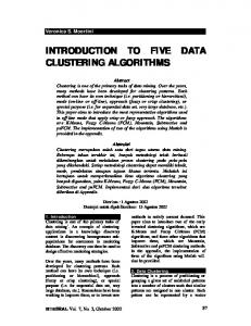
Figure 1: System diagram of a spectral feature speaker recognizer, the focus of this study. Clustering methods are characterized here by their clustering quality, resulting speaker recognition accuracy, time consumption of the modeling, and usability aspects. There are two common ways to train speaker models, (a) maximum likelihood (ML) that trains the model using feature vectors of the speaker, and (b) maximum a posteriori (MAP) that uses in addition a universal background model (UBM) to generate a robust model.
Speaker recognition process is illustrated in Fig. 1. When a new person is enrolled into the system, the audio signal is first converted into a set of feature vectors. Although short-term spectral features [34] are sensitive to noise and channel effects, they provide better recognition accuracy than prosodic and “high-level” features [69], and are therefore used in this study. Following feature extraction, a speaker model is trained and added into the database. In the matching phase, feature vectors are extracted from the unknown sample and compared with the model(s) in the database, providing a similarity score. To increase robustness to signal variability, recent solutions use sophisticated speaker model compensation [7, 41] and score normalization using background speakers [1, 68]. Finally, the normalized score is compared with a threshold (verification), or the best scoring speaker(s) is selected as such (identification). A number of different classifiers have been studied for speaker recognition; see [66, 42] for an overview. Speaker models can be divided into generative and discriminative models. Generative models characterize the distribution of the feature vectors within the classes (speakers), whereas discriminative modeling focuses on modeling the decision boundary between the classes. For generative modeling, vector quantization (VQ) [8, 28, 32, 45, 74, 80] and Gaussian mixture model (GMM) [67, 68] are commonly used. For
discriminative training, artificial neural networks (ANNs) [17, 83] and, more recently, support vector machines (SVMs) [10, 11] are representative techniques. In the past few years, research community has also focused on combining generative and discriminative models, leading to hybrid models. In particular, GMMs are extensively used for mapping variable-length vector sequences into fixed-dimensional supervectors [11, 13, 49] that are used as features in SVM. Parallel to, and in conjunction with this research trend, significant recent advances have also been made on intersession variability compensation of the supervectors [7, 13, 41]. A representative class of such techniques is factor analysis (FA) model in the GMM supervector space [13, 41]. Both the hybrid GMM-SVM approaches and the factor analysis models have excellent performance especially under severe channel and session mismatches. However, due to the additional training steps required for constructing the GMM front-end and, subsequently, the session variability models, the supervector methods typically require at least an order of magnitude more development data compared to traditional generative models [30, 32, 68], and are therefore much more CPU-intensive. Careful selection of the various modeling data sets is also a critical step 1.
1.1 Relevance of Clustering in a Large-Scale Pattern Recognition Problem In this paper, we focus on the training methodology of two classical generative speaker models, GMM and VQ, for two reasons. Firstly, these methods underlie both the traditional maximum likelihood (or minimum distortion) trained speaker models [8, 28, 45, 74, 80], their maximum a posteriori adapted extensions using universal background model (UBM) priors [30, 32, 68] and, importantly, also the recent hybrid GMM-SVM and FA models [11, 13, 41, 49]. The way the underlying generative model is trained will have a major effect to the performance of all these methods. Secondly, while there are good guidelines for composing a balanced and representative training set for background modeling – see the recent study [30] and references therein – the question of how to model the generative model itself has received only little attention in literature. Typically, Gaussian mixture models, which are pertinent not only in speaker recognition but in all speech applications and general audio classification tasks [2], are trained using the expectation-maximization (EM) algorithm, or, in the case of vector quantization, the Kmeans algorithm. Better clustering algorithms have been introduced after K-means and EM [37], in terms of preventing local minima, being less sensitive to parameter setup and providing faster processing. Even though several literature surveys exist [36, 37, 60, 77], only a few extensive comparisons are available in image processing [24] and text retrieval [76] but none in speaker recognition. In clustering research, new methods are usually compared in 1
In practice, the various datasets need to be selected according to the expected conditions of the actual application data, reflecting the channel conditions, noise levels, as well as the speaker population (e.g. native language of speakers). Additional care must be taken when the same speakers (but possibly different utterances) are re-used in background modeling and score normalization. The degrees of variability used in the NIST speaker recognition evaluation datasets (http://nist.gov/itl/iad/mig/sre.cfm) increases every year and proper selection of training datasets is critical.
terms of clustering quality. But should better clustering quality improve the recognition accuracy of the full pattern recognition system? Overall, given the long history of clustering research [37], existence of thousands of clustering methods, we feel that it is time to review the choice of clustering methodology in a large-scale, real-world pattern recognition problem involving tens of dimensions and hundreds of pattern classes of highly noisy data. In our view, text-independent speaker recognition is a representative application. The main goal of this paper is to bridge some of the gap between theoretical clustering research and large-scale pattern recognition applications, by focusing to an important practical design question: choice of clustering methodology. Before representing the research hypotheses, we first review the role of GMM and VQ clustering methods in our target application.
1.2 Review of Clustering Methods in Speaker Recognition The VQ model (centroid model) is a collection of prototype vectors determined by minimizing a distance-based objective function. GMM is a model-based approach [59] where the data is assumed to follow Gaussian mixture distribution parameterized by mean vectors, covariance matrices and mixing weights. For a fixed number of clusters, GMM has more free parameters than VQ. Their main difference is the cluster overlap in GMM. In fact, VQ can be seen as a special case of the GMM in which the posterior probabilities have been hardened, and unit variance is assumed in all clusters. Similarly, k-means algorithm [52] can be considered as a special case of the expectation maximization (EM) algorithm for GMM [5]. The VQ model was first introduced to speaker recognition in [8, 74] and the GMM model in [67]. GMM remains a core component in state-of-the-art speaker recognition whereas VQ is usually seen as a simplified variant of GMM. GMM combined with UBM [68] is the de facto reference method (Fig. 1b). The role of VQ, on the other hand, has been mostly in reducing the number of training or testing vectors to reduce the computational overhead. VQ has also been used as a pre-processor for ANN and SVM classifiers in [54, 81] to reduce the training time and for speeding up the GMM-based verification in [45, 70]. In [50], VQ is used for partitioning the feature space into local decision regions modeled by SVMs to increase accuracy. Despite its secondary role, VQ gives comparable accuracy to GMM [6, 46] when equipped with a MAP adaptation [32]. The computational benefits over GMM are important in small-footprint implementations such as mobile devices [71]. Recently, similar to hybrids of GMM and SVM [11], combination of VQ with SVM has also been studied [6]. Fuzzy clustering [15] is a compromise between VQ and GMM models. It retains the simplicity of VQ while allowing soft cluster assignments using a membership function. Fuzzy extensions of both VQ [80] and GMM [79] have been studied in speaker recognition. For a useful review, refer to [78]. Another recent extension of GMM is based on nonlinear warping of the GMM density function [82]. These methods, however, lack formulation for the background model adaptation [68], which is an essential part of modern speaker verification relying on MAP training (Fig. 1b). The model order – number of centroid vectors in VQ or Gaussian components in GMM – is an important control parameter in both VQ and GMM. Typically the number varies
from 64 to 2048, depending on the chosen features and their dimensionality, number of training vectors, and the selected clustering model (VQ or GMM). In general, increasing the number of clusters improves recognition accuracy, but it levels off after a certain point due to over-fitting. From the two clustering models, VQ was found to be less sensitive to the choice of the number of clusters in [75] when trained without the UBM adaptation. The model order in both VQ and GMM needs to be carefully optimized for the given data to achieve good performance [46]. The choice of the clustering method, on the other hand, has been much less studied. Usually K-means [52] and expectation-maximization (EM) [5, 57] methods have been used, although several better clustering methods exist [24]. This raises the questions of which clustering algorithm should be chosen, and whether the choice between VQ or GMM model matters. Regarding the choice between these models, experimental evidence is diverse. GMM has been shown to perform better for small model orders [75], but the difference vanishes when using larger model order [28, 45, 75]. However, GMM has been reported to work better than VQ only when cluster-dependent covariance matrices were used but perform worse when a shared covariance matrix was used [67]. Several authors have used GMM derived from the VQ model for faster training [47, 63, 73]. All these observations are based on the maximum likelihood (ML) training of speaker models though. Two recent studies include more detailed comparisons of GMM and VQ [46, 29]. In [46] the MAP trained VQ outperformed MAP-trained GMM for longer training data (2.5 minutes) but the situation was reversed for 10-second speech samples. The study of [29] focused on the choice of dissimilarity measure (city-block, euclidean, Chebychev) in VQ and two different clustering initializations (binary LBG splitting [52] versus random selection). Differences in the identification and verification tasks, as well as ML versus MAP training were also considered. The authors found the distance measure and the number of clusters to be more important than the choice of the K-means initialization. ML-trained models performed better with the shorter NTIMIT data in speaker identification, whereas MAP-trained models (both GMM and VQ) worked better on longer training segments (NIST 2001). Regarding the choice between GMM and VQ, they performed equally well on the NIST 2001 verification task, regardless whether trained by ML or MAP. However, in the identification task, MAP-trained GMM outperformed MAP-trained VQ, on both corpuses. A recent study [6] compares MAP-trained GMM and VQ models when used as front-end features for SVM. From the two corpuses, GMM variant outperformed VQ on the YOHO corpus with short utterances, whereas VQ performed slightly better on the KING corpus with longer free-vocabulary utterances.
1.3 Research Objectives and Hypotheses Existing literature lacks extensive comparison between different clustering algorithms that would be useful for practitioners. The existing comparisons in speaker recognition study only a few methods, use different features and datasets preventing meaningful cross-comparisons. Even in [29, 46], only the basic EM and K-means algorithms were studied. Thus, extensive comparison of better clustering algorithms is still missing.
In the experimental section of this paper, we consider the GMM and VQ models both in the maximum likelihood (ML) and maximum a posteriori (MAP) training setting, without additional SVM back-end, inter-session compensation or score normalization [1]. Focusing on this computationally feasible core component enables detailed study of generative model training methodology without re-training the full recognition system from scratch every time the background models are changed; the same rationale was chosen recently in [30]. In the experiments, we consider both controlled laboratory quality speech (TIMIT corpus) and noisy conversional telephony speech (NIST 1999 and NIST 2006 corpuses). Our main evaluation criteria are the recognition accuracy, processing time and ease of implementation. We aim at answering the following questions: 1. Is clustering needed or would random sub-sampling be sufficient? 2. What is the best algorithm in terms of quality, efficiency and simplicity? 3. What is the difference between the accuracy of the VQ and GMM models? It was hypothesized in [43] that a clustering would be required but the choice of clustering algorithm would not be critical. A possible explanation is that the speech data may not have a clustering tendency [44]. These observations were based on a small 25speaker laboratory-quality data collected using the same microphone and read sentences. In this paper, we aim at confirming these hypotheses via extensive large scale experiments. Since the main advantage of speaker recognition over other biometric modalities is possibility for low-cost remote authentication, we experiment using realistic telephony data including different handsets, transmission lines, GSM coding and environmental noises. The two NIST corpuses used in the study include 290,521 (NIST 1999) and 53,966 (NIST 2006) verification trials including 539 and 816 speakers, respectively. Furthermore, in NIST 2006 corpus, all the verification trials are from highly mismatched channel conditions. This makes it a very challenging pattern recognition problem. Regarding the difference between the VQ and GMM models, our results reveal insights which are not obvious, and sometimes contradict previous understanding based on literature. For example, even though the models are of similar quality in terms of average speaker verification accuracy (equal error rate), their performance differs systematically at the extreme cases where small false acceptance or false rejection errors are required.
2 CLUSTERING MODELS AS SPEAKER MODELS 2.1 Problem formulation We consider a training set X = {x1,…,xN}, where x i = ( xi(1) ,..., xi( d ) ) ∈ R d are the ddimensional feature vectors. In the centroid-based model, also known as the vector quantization (VQ) model, the clustering structure is represented by a set of code vectors known as the codebook, which is denoted here as C = {c1,…cK}, where K