Clustering Driven Cascade Classifiers for Multi-Indexing of Polyphonic Music by Instruments Wenxin Jiang, Zbigniew W. Ra´s, Alicja A. Wieczorkowska
Abstract Recognition and separation of sounds played by various instruments is very useful in labeling audio files with semantic information. Numerous approaches on acoustic feature extraction have already been proposed for timbre recognition. Unfortunately, none of these monophonic timbre estimation algorithms can be successfully applied to polyphonic sounds, which are more usual cases in the real music world. This has stimulated the research on a hierarchically structured cascade classification system under the inspiration of the human perceptual process. This cascade classification system makes first estimate on the higher level of the decision attribute, which stands for the musical instrument family. Then, the further estimation is done within that specific family range. However, the traditional hierarchical structures were constructed in human semantics, which are meaningful from human perspective but not appropriate for the cascade system. We introduce the new hierarchical instrument schema according to the clustering results of the acoustic features. This new schema better describes the similarity among different instruments or among different playing techniques of the same instrument. The classification results show a higher accuracy of cascade system with the new schema compared to the traditional schemas.
Wenxin Jiang University of North Carolina, Dept. of Computer Science, Charlotte, NC 28223, USA e-mail:
[email protected] Zbigniew W. Ra´s University of North Carolina, Dept. of Computer Science, Charlotte, NC 28223, USA & PolishJapanese Institute of Information Technology, Koszykowa 86, 02-008 Warsaw, Poland e-mail:
[email protected] Alicja A. Wieczorkowska Polish-Japanese Institute of Information Technology, Koszykowa 86, 02-008 Warsaw, Poland email:
[email protected]
1
2
Wenxin Jiang, Zbigniew W. Ra´s, Alicja A. Wieczorkowska
1 Introduction Different classifiers have been used in musical instrument estimation domain, usually for a small number of instruments [1], [7], [12]. Still, it is a non-trivial problem to choose the one with the optimal performance in terms of estimation accuracy for most western orchestral instruments. It is common to try different classifiers on the same training database which contains the features extracted from audio files and select the classifier which yields the highest accuracy for the training database. The selected classifier is used for the timbre estimation on analyzed music sounds. There are also boosting systems [3], [2] consisting of a set of weak classifiers and iteratively adding them to a final strong classifier. Boosting systems usually achieve a better estimation model by training each given classifier on a different set of samples from the training database, which uses the same number of features (attributes). In other words, boosting system works under assumption that there is a (big) difference between different groups of subsets of the training database, so different classifiers are trained on the corresponding subset based on their expertise. However, due to the homogeneous characteristics across all the data samples in a training database, musical data usually cannot take full advantage of such panel of learners because none of the given classifiers would get a majority weight. Thus the improvement cannot be achieved by such a combination of different classifiers. Also, in many cases, the speed of classification is also an important issue. To achieve the applicable classification time while preserving high classification accuracy, we introduce the cascade classifier which may further improve the instruments’ recognition of the MIR system. Cascade classifiers have been investigated in the domain of handwritten digit recognition. Thabtah [18] used filter-and-refine processes and combined it with kNearest Neighbor (KNN) classifier to give the rough but fast classification with lower dimensionality of features at filter step and to rematch the objects marked by the previous filter with higher accuracy by increasing dimensionality of features. Also, Lienhart [8] used CART trees as base classifiers to build a boosted cascade of simple feature classifiers to achieve rapid object detection. It is possible to construct a simple instrument family classifier with a low recognition error, which is called a classification pre-filter. When one musical frame is labeled by a specific family, the training samples in other families can be immediately discarded, and further classification is then performed within small subsets, which could be identified by a stronger classifier through adding more features or even calculating the complete spectrum. Since the number of training samples is reduced, the computational complexity is reduced while the recognition rate still remains high.
Classifiers for Multi-Indexing of Polyphonic Music by Instruments
3
2 Hierarchical structure of musical instrument sound classification According to the experience regarding human recognition of musical instruments, it is usually easier for one to tell the difference between violin and piano than violin and viola. This is because violin and piano belong to different instrument families and thus have quite different timbre qualities. Violin and viola fall into the same instrument family which indicates they share quite similar timbre quality. If we build the classifiers both on the family level and the instrument level, then the polyphonic music sound is first classified at the instrument family level. After a specific instrument family label is assigned to the analyzed sound by the classifier, it can be further classified at the instrument level by another classifier which is built on the training data of that specific instrument family. Since there is a smaller number of possible instruments in this family, the classifier trained on this family has the appropriate expertise for the classification of the instruments within it. Before we discuss how to build classifiers on different levels, let us first have a look at the hierarchical structure of the western instruments. Erich von Hornbostel and Curt Sachs published an extensive scheme for musical instrument classification in 1914. Their scheme is widely used today, and is most often known as the Hornbostel-Sachs system. Figure 1 shows a part of the Hornbostel/Sachs instrument classification tree. The Hornbostel-Sachs system includes aerophones (wind instruments), chordophones (string instruments), idiophones (made of solid, nonstretchable, resonant material), and membranophones (mainly drums). Idiophones and membranophones are called percussion. Additional groups include electrophones, i.e. instruments where the acoustical vibrations are produced by electric or electronic means (electric guitars, keyboards, synthesizers), complex mechanical instruments (including pianos, organs, and other mechanical music makers), and special instruments (include bullroarers, but they can be classified as free aerophones). Each category can be further subdivided into groups, subgroups etc. and finally into instruments. Idiophones’ subcategories include instruments classified as: struck (e.g. gongs), struck together (by concussion - e.g. claves, clappers, castanets, finger cymbals), scrapped, rubbed, stamped, shaken (e.g. rattles), and plucked (e.g. Jew’s harp). Membranophones include the following subgroups: cylindrical drum, conical drum, barrel drum, hourglass drum, goblet drum, footed drum, long drum, kettle or pot drum, frame drum (e.g. tambourine), friction drum, and mirliton/kazoo. Chordophones’ subcategories include: zithers, lutes plucked (e.g. mandolins, guitars, ukuleles), lutes bowed (e.g. viols - fretted neck, fiddles, violin, viola, cello, double bass, and hurdy-gurdy - no frets), and harp. Aerophones are classified into the following subgroups: free aerophone (e.g. bullroarers), end-blown flute, sideblown flute, nose flute, globular flute (e.g. ocarina), multiple flutes, Panpipes, whistle mouthpiece (e.g. recorder), air chamber (e.g. accordion); single reed instruments (such as clarinet, saxophones), double reed (such as oboe, bassoon) and lip vibrated (trumpet or horn) - instruments classified according to the mouthpiece used to set air in motion to produce sound. Some of Aerophones subcategories are also called
4
Wenxin Jiang, Zbigniew W. Ra´s, Alicja A. Wieczorkowska
woodwinds (single reed, double reed, flutes) or brass (lip vibrated), but this criterion is not based on the material the instrument is made of, but rather on the method of sound production. In woodwinds, the change of pitch is mainly obtained by the change of the length of the column of the vibrating air. Additionally, over-blow is applied to obtain second, third or fourth harmonic to become the fundamental. In brass instruments, over-blows are very easy because of wide bell and narrow pipe, and therefore over-blows are the main method of pitch changing.
All
aerophone
idiophone
aero_double-reed
aero_lip-vibrated
aero_single-reed
Instrument level
Instrument level
Instrument level
94%
94%
94%
chordophone
Fig. 1 A part of the Hornbostel-Sachs hierarchical tree
Sounds can be also classified according to the articulation, i.e. the method the instrument is played. According to articulation, sounds can be basically classified in the following 3 ways: (1) sustained or non-sustained sounds, (2) muted or not muted sounds, (3) vibrated and not vibrated sounds. This classification may be difficult, since the vibration may not appear in the entire sound; some changes may be visible, but no clear vibration. Also, brass is sometimes played with moving the mute in and out of the bell. According to MPEG7 classification [9], there are four classes of musical instrument sounds: (1) Harmonic, sustained, coherent sounds well detailed in MPEG7, (2) Non-harmonic, sustained, coherent sounds, (3) Percussive, non-sustained sounds - well detailed in MPEG7, (4) Non-coherent, sustained sounds. Musical instruments may produce sound of definite or indefinite pitch. Still, most of musical instrument sounds of definite pitch have some noises/continuity in their spectra. In our experiments, we do not include membranophones because the instruments of this family usually do not produce the harmonic sound, so they need special techniques to be identified. This chapter focuses on the instruments producing basically harmonic sounds. Figure 2 shows another tree structure of instrument sound classification, in which sounds are grouped according to the way how the musical instruments are played.
Classifiers for Multi-Indexing of Polyphonic Music by Instruments
5
Fig. 2 A part of the play method (articulation) hierarchical tree
3 MIR Framework based on cascade classification system In this section, we describe cascade classification strategy investigated for musical instruments estimation [15]. Based on how the hierarchical instrument family structures, we have implemented the cascade classification system for the polyphonic sound estimation, as shown in the Figure 3.
Fig. 3 Timbre estimation with classifier and feature selection
Let S = {F,C, D} be the multiple-classifier timbre estimation system, where D = {d1 , . . . , dn } is the set of all possible decision values of musical instruments in S , F = { f1 , . . . , fm } is the collection of all available feature sets which could be extracted from the input signal and then used by the classifiers to identify the target frame. C = {C1 , . . . ,Cw } is the set of classifiers built on feature sets F after they are extracted from the standard instrument sounds and saved as the feature training database. Let X = {x1 , . . . , xt } be the set of segmented frames from the input au-
6
Wenxin Jiang, Zbigniew W. Ra´s, Alicja A. Wieczorkowska
dio sound. There are multiple processes of classification for each frame xt . First at the root of the hierarchical tree, then down to its lower level, we have pairs (Cz , fy ), 1 ≤ z ≤ w, 1 ≤ y ≤ m, where (Cz , fy ) means ”use classifier Cz on the feature set fy ”, to perform classification at each level and get the estimation confidence, i.e. the probability of the classification result given by classifier (related to the similarity between the analyzed frame and reference frames), con f (xi , α ) = Cz ( fy ), where α is the specific node of the tree. The result should satisfy two constraints: con f (xi , α ) ≥ λ1 and sup(xi , α ) ≥ λ2 , where λ1 is the minimum confidence for the correct classification and λ2 is the threshold for minimal support (λ1 and λ2 are given by the user). Support is defined as the number of matched frames of a particular instrument from the reference database (during classification process, the algorithm tries matching frames to all available frames representing all instruments in the database, and the most similar ones are returned as the matched frames). Confidence is the ratio of support over the total number of matched frames. After classifications are finished at all the levels, we get the final instrument estimations {d p } for the frame xi (multiple instrument estimations are given by classifier for each frame), where d p ∈ D, and the overall confidence for each instrument estimation is calculated by multiplying the confidence obtained previously at each classification level con f (xi , d p ) = ∏αv =1 con f (xi , α ),where v is the total number of ancestors for node xi in the path of hierarchical tree. After all the individual frames are estimated by the classification system, a smoothing process is performed within a smoothing window. It is done by calculating the average confidence for each possible instrument within the window con f (d p ) = ∑sq=1 con f (d p )q /s where s is the size of a smoothing window. The smoothing window is an indexing granule, which is the smallest segment of the signal on which the estimation of instruments is yielded by the indexing system - the indexing system yields the list of instruments for each smoothing window instead of each frame; the smoothing window size usually is 1-2 seconds, whereas the analyzing frame is 0.12 second, which would be rather short for such labeling, and too short for the users to estimate instruments by themselves. Next, the output of the final results is further controlled by the threshold λ3 . If the mean value of the confidence within smoothing window con f (d p ) > λ3 , where λ3 is given by the user, the instrument candidate is kept, otherwise it is discarded as the noise signal which only occurs in a very short time period. According to the indexing resolution requirement, smoothing window can be adjusted to the desired size. The advantage of this process is that it uses the information of music context to further adjust the results from the frame-wise estimation phase. The system will perform timbre estimation for the polyphonic sound with high accuracy while still preserving the applicable analyzing speed by choosing the best feature and classifier for the classification process at each level based on the knowledge derived from the training database.
Classifiers for Multi-Indexing of Polyphonic Music by Instruments
7
4 Hierarchical Structure Based on Clustering Analysis Clustering is the classification of data objects into similarity groups (clusters) according to a defined distance measure. It is widely used as one of the important techniques of machine learning and pattern recognition in such fields as biology, genomics and image analysis. However, it has not been well investigated in the music domain, since the category information of musical instruments has already been defined by musicians as the two hierarchical structures demonstrated in the previous section. These structures group the musical instrument sounds according to their semantic similarity which is concluded from the human experience. However, the instruments that are assigned to the same family or subfamily by these hierarchical structures often sound quite different from another. On the other hand, instruments that have similar timbre qualities can be assigned to very different groups by these hierarchical structures. Thus, the inconsistency between the timbre quality and the family information causes the incorrect timbre estimation, given by the cascade classification system based on Hornbostel-Sachs instrument classification, used in our previous research [5]. For instance, the trombone belongs to the aerophone family, but the system often classifies it as the chordophone instrument, such as violin. In order to take the full advantage of the cascade classification strategy, we have built a new hierarchical structure of musical instruments by the matching learning technique. Cluster analysis is commonly used to search for groups in data. It is most effective when the groups are not known a priori. We use the cluster analysis methods to re-organize the instrument groups according to the similarity of timbre relevant features among the instruments.
4.1 Clustering analysis methods There exist many clustering algorithms. Basically, all the clustering algorithms can be divided into two categories: partitional clustering and hierarchical clustering. Partitional clustering algorithms determine all clusters at once without hierarchical merging or dividing process. K-means clustering is most common method in this category [11]; K is the empirical parameter. Basically, it randomly assigns instances to K clusters. Next, new centroid for each of the K clusters and the distance of all items to these K centroids are calculated. Items are re-assigned to the closest centroid and the whole process is repeated until cluster assignments are stable. Hierarchical clustering generates a hierarchical structure of clusters which may be represented in a structure called dendrogram. The root of the dendrogram consists of a single cluster containing all the instances, and the leaves correspond to individual instances. Hierarchical clustering can be further divided into two types according to whether the tree structure is constructed by following agglomerative or divisive approach. Agglomerative approach works in the bottom-up manner, it recursively merges smaller clusters into larger ones till some stoping condition is reached. Algo-
8
Wenxin Jiang, Zbigniew W. Ra´s, Alicja A. Wieczorkowska
rithms based on divisive (or top-down) approach begin with the whole set and then recursively split this set into smaller ones till some stoping condition is reached. We have chosen the hierarchical clustering method to learn the new hierarchical schema for music instruments, since it fits our scenario well. There are many options to compute the distance between two clusters. The most common methods are the following [19]: • Single linkage (nearest neighbor). In this method, the distance between two clusters is determined by the distance of the two closest objects (nearest neighbors) in different clusters. This rule will string objects together to form the clusters, and the resulting ones tend to represent long ”chains”. • Complete linkage (furthest neighbor). In this method, the distances between clusters are determined by the greatest distance between any two objects in different clusters (the ”furthest neighbors”). This method usually performs quite well in cases when the objects actually form naturally distinct ”clumps.” If the clusters tend to be of a ”chain” type, then this method is inappropriate. • Unweighted pair-group method using arithmetic averages (UPGMA). In this method, the distance between two clusters is calculated as the average distance between all pairs of objects in two different clusters. This method is also very efficient when the objects form natural distinct ”clumps” and it performs equally well with ”chain” type clusters. • Weighted pair-group method using arithmetic averages (WPGMA). This method is identical to the UPGMA method, except that in the computations, the size of the respective clusters is used as a weight. Thus, this method should be used when the cluster sizes are suspected to be greatly uneven [17]. • Unweighted pair-group method using the centroid average (UPGMC). The centroid of a cluster is the average point in the multidimensional space, calculated as the mean value (for each dimension separately). In a sense, it is the center of gravity for the respective cluster. In this method, the distance between two clusters is determined as the difference between centroids. • Weighted pair-group method using the centroid average (WPGMC). This method is identical to the previous one, except that weighting is introduced into the computation. When there are considerable differences in cluster sizes, this method is preferable to the previous one. • Ward’s method. This method is distinct from all other methods because it uses an analysis of variance approach to evaluate the distances between clusters. In short, this method attempts to minimize the Sum of Squares of any two hypothetical clusters that can be formed at each step. In general, this method is good at finding compact, spherical clusters. However, it tends to create clusters of small size. To complete the above definitions of a distance measure between two clusters, we also have to define the distance between their instances or centroids. Here are some most common distance measures between two objects: 1. Euclidean: Usual square distance between the two vectors. Disadvantages: not scale invariant, not for negative correlations
Classifiers for Multi-Indexing of Polyphonic Music by Instruments
9
p dxy = ∑ (xi − yi )2 2. Manhattan: Absolute distance between the two vectors. dxy = ∑ |xi − yi | 3. Maximum: Maximum distance between any two components of x and y dxy = max|xi − yi | 4. Canberra: Canberra distance examines the sum of series of a fraction differences between coordinates of a pair of objects. Each term of fraction difference has value between 0 and 1. If one of coordinates is zero, the term corresponding to this coordinate become unity regardless the other value, thus the distance will not be affected; if both coordinates are zero, then the term is defined as zero. −yi | dxy = ∑ |x|xi i|+|y i| 5. Pearson correlation coefficient (PCC) is a correlation-based distance. It measures the degree of association between two variables.
ρxy =
[cov(X,Y )]2 var(X)var(Y )
, dxy = 1 − ρxy where cov(X,Y ) is the covariance of the two
variables, var(X) and var(Y ) - the variance of each variable. 6. Spearman’s rank correlation coefficient is another correlation based distance. 6 d2
i ρxy = 1 − n(n∑2 −1) , dxy = 1 − ρxy
where di = xi − yi is the difference between the ranks of corresponding values xi and yi , and n is the number of values in each data set (same for both sets). Rank is calculated in the following way: 1 is assigned to the smallest element of each data, 2 to the second smallest element, and so on; the average ranking is calculated if there is a tie among different elements. It is critical to choose an appropriate distance measure for objects in a musical domain because different measures may produce different shapes of clusters which represent different schema of instrument family. Different features also require the appropriate measures to be chosen in order to give better description of feature variation. The inappropriate measure could distort the characteristics of timbre which may cause the incorrect clustering.
4.2 Evaluation of different clustering algorithms for different features As we can see, each clustering method has its own different advantage and disadvantage over others. It is a nontrivial task to decide which one is the most appropriate method for generating the hierarchical instrument classification structure. Not only the specific cluster linkage method needs to be decided in the hierarchical clustering algorithms, but also the good distance measurement has to be chosen in order to generate the good schema that represents the actual relationships among those instruments. We designed quite intensive experiments with the ”cluster” package
10
Wenxin Jiang, Zbigniew W. Ra´s, Alicja A. Wieczorkowska
in R system [14]. The R package provides two hierarchical clustering algorithms: hclust (agglomerative hierarchical clustering), and diana (divisive hierarchical clustering). Table 1 shows all the clustering methods that we tested. We evaluated six different distance measurements (Euclidean, Manhattan, Maximum, Canberra, Pearson correlation coefficient, and Spearman’s rank correlation coefficient) for each algorithm. For the agglomerative type of clustering (hclust), we also evaluated seven different cluster linkages that are available in this package: Ward, single (single linkage), complete (complete linkage), average (UPGMA), mcquitty (WPGMC), median(WPGMA), and centroid (UPGMC). Table 1 All distance measures and linkage methods tested for agglomerative and divisive clustering Clustering algorithm
Cluster Linkage
Distance Measure
hclust (agglomerative)
average centroid complete mcquitty median single ward
6 distance metrics 6 distance metrics 6 distance metrics 6 distance metrics 6 distance metrics 6 distance metrics 6 distance metrics
diana (divisive)
N/A
6 distance metrics
We have chosen the middle C pitch group which contains 46 different musical sound objects. We have extracted three different feature sets (MFCC [10], spectral flatness coefficients [9], and harmonic peaks [9]) from those sound objects. Each feature set produces one dataset for clustering. Some sound objects belong to the same instrument. For example, ”ctrumpet” and ”ctrumpet harmonStemOut” are objects produced by the same instrument: trumpet. We have preserved these particular object labels in our feature database without merging them as the same label because they could have very different timbre quality which the conventional hierarchical structure ignores. We have tried to discover the unknown musical instrument group information solely by the unsupervised machine learning algorithm, instead of applying any human guidance. Each sound object was segmented into multiple 0.12s frames and each frame was stored as an instance in the testing dataset. Since the segmentation is performed with overlap of 2/3 of the frame, there were totally 2884 frames from the 46 objects in each of the three feature datasets. When our algorithm finishes the clustering job, a particular cluster ID is assigned to each frame. Theoretically, one may expect the same cluster ID to be assigned to all the frames of the same instrument sound object. However, the frames from the same sound object are not uniform and have variations in their feature patterns as the time evolves. Therefore, clustering algorithms do not perfectly identify them as the same cluster. Instead, some frames are assigned into other groups where majority
Classifiers for Multi-Indexing of Polyphonic Music by Instruments
11
of the frames come from other instrument sounds. As a result, multiple (different) cluster IDs are assigned to the frames of the same instrument object. Our goal is to cluster the different instruments into the groups according to the similarity of timbre relevant features. Therefore, one important step of the evaluation is to check if a clustering algorithm is able to cluster most frames of an individual instrument sound into one group. In other words, a clustering algorithm should be able to differentiate most of the frames of one instrument sound from the others. It is evaluated by calculating the accuracy of a cluster ID assignment. We use the following example to illustrate this evaluation process. A hierarchical cluster tree Tm is produced by a clustering algorithm Am . There are totally n instrument sound objects in the dataset (n=46). The clustering package provides function cutree to cut Tm into n clusters. One of these clusters is assigned to each frame. Table 2 shows a contingency table (xi j represent numbers) derived from the clustering results after the cutree is applied. It is a n × n matrix, where xi j is the number of frames of instrumenti that are labeled by cluster j , and xi j ≥ 0. Table 2 Format of the contingency table derived from clustering result
Instrument1 ··· Instrumenti ··· Instrumentn
Cluster1
···
Cluster j
···
Clustern
x11 ··· xi1 ··· xn1
··· ··· ··· ··· ···
x1 j ··· xi j ··· xn j
··· ··· ··· ··· ···
x1n ··· xin ··· xnn
In order to calculate the accuracy of the cluster assignment, we need to decide which cluster ID corresponds to which instrument object. If cluster k is assigned to instrumenti , xik is the number of correct assignments for instrumenti , the accuracy of the clustering for instrumenti is βi = xik /(∑nj=1 xi j ). During clustering process, each frame of the sound object is clustered into one particular group, and the group ID (i.e. instrument) is assigned to this frame. For each row, the maximum value is found among n columns, and next the column corresponding to the position of this maximum becomes the class label for frames represented in this row. However, it may happen that the maximum value is found in the same column also for other rows, and then the same group ID is linked to two different sound objects, which means these two different instrument sounds could not be distinguished by this particular clustering scheme. Clearly, we would like to avoid such an ambiguity. On the other hand, we have to cluster many frames of one sound object into a single group. Therefore, we would need permutations to calculate the theoretic best solution for the whole table, but such a large number of computations cannot be performed. The overall accuracy for the clustering algorithm Am is the average accuracy of all the instruments β = (∑ni=1 βi )/n. To find the maximum β among all possible cluster assignments to instruments, we should permute this matrix in order to find
12
Wenxin Jiang, Zbigniew W. Ra´s, Alicja A. Wieczorkowska
the maximum accuracy for the whole matrix (for each row of matrix, there are multiple values that could be selected among n columns), but it is not applicable to perform such a large number of calculations. This is why we have chosen maximum xi j in each row to approximate the optimal β . Since it is possible to assign the same cluster to multiple instruments, we have taken the number of clusters as well as accuracy into account. The final measurement to evaluate the performance of clustering is scorem = β · w, where w is the number of clusters, w ≤ n. This measure reflects how well the algorithm clusters the frames from the same instrument object into the same cluster. It also reflects the ability of algorithm to separate instrument objects from each other. In the experiments, we used two hierarchical clustering algorithms, hclust and diana. Table 3 presents 15 results which yielded the highest score among 126 experiments based on hclust algorithm. Table 3 Evaluation result of hclust algorithm Feature
method
metric
β¯
w
score
Flatness Coefficients Flatness Coefficients Flatness Coefficients mfcc mfcc Flatness Coefficients mfcc mfcc mfcc Flatness Coefficients Flatness Coefficients mfcc Flatness Coefficients mfcc
ward ward ward ward ward ward ward ward ward ward ward ward mcquitty ward
pearson euclidean manhattan kendall pearson kendall euclidean manhattan spearman spearman maximum maximum euclidean average
87.3% 85.8% 85.6% 81.0% 83.0% 82.9% 80.5% 80.1% 81.3% 83.7% 86.1% 79.8% 88.9% 87.3%
37 37 36 36 35 35 35 35 34 33 32 34 33 30
32.30 31.74 30.83 29.18 29.05 29.03 28.17 28.04 27.63 27.62 27.56 27.12 26.67 26.20
From the results, the Ward linkage outperforms other methods and it yields the best performance when Pearson distance measure is used on the flatness coefficients feature dataset. Table 4 shows the results from diana algorithm. In this algorithm, Euclidean yields the highest score on the mfcc feature dataset. During the clustering process, we cut the hierarchical clustering result at a certain level, when obtaining groups which could represent instrument objects. If most of the frames from the same instrument object are clustered into one group, then this algorithm is selected to generate the hierarchical tree. When we compare the two algorithms (hclust and diana), hclust yields better clustering results than diana. Therefore, we chose agglomerative clustering algorithm to generate the hierarchical schema for musical instruments, using Ward as the linkage method, Pearson distance measure as the distance metric, and Flatness Coefficients as the feature dataset to perform clustering analysis.
Classifiers for Multi-Indexing of Polyphonic Music by Instruments
13
Table 4 Evaluation result of diana algorithm Feature
metric
β¯
w
score
Flatness Coefficients Flatness Coefficients Flatness Coefficients Flatness Coefficients Flatness Coefficients mfcc mfcc mfcc mfcc mfcc
euclidean kendall manhattan maximum pearson euclidean kendall manhattan pearson spearman
77.3% 75.7% 76.8% 80.3% 79.9% 78.5% 77.2% 77.7% 83.4% 81.2%
24 23 25 23 26 29 27 26 25 24
18.55 17.40 19.20 18.47 20.77 22.78 20.84 20.21 20.86 19.48
5 New hierarchical tree Figure 4 shows the dendrogram result generated by the hierarchical clustering algorithm we chose (i.e. agglomerative clustering), as mentioned in Section 4.2. From this new hierarchical classification, we discover some instrument relationships which are not represented in the traditional schemas. A musical instrument can produce sounds with quite different timbre qualities when different playing techniques are applied. One of the common techniques is muting. A mute is a device fitted to a musical instrument to alter the sound produced. It usually reduces the volume of the sound as well as affects the timbre. There are several different mute types for different instruments. The most common type used with the brass is the straight mute - a hollow, cone-shaped mute that fits into the bell of the instrument. This results in a more metallic, sometimes nasal sound, and when played at loud volumes can result in a very piercing note. The second common brass mute is the cup mute. Cup mutes are similar to straight mutes, but attached to the end of the mute’s cone is a large lip that forms a cup over the bell. The result is removal of the upper and lower frequencies and a rounder, more muffled tone. In the case of string instruments of the violin family, the mute takes the form of a comb-shaped device attached to the bridge of the instrument, dampening vibrations and resulting in a ”softer” sound. In the hierarchical structure shown in Figure 4, ”trumpet” and ”ctrumpet harmonStemOut” represent two different sounds produced by the trumpet. ”ctrumpet harmonStemOut” is produced when a particular mute is applied, called Harmon mute (different from the common straight or cup mutes). It is a hollow, bulbous metal device placed in the bell of the trumpet. All air is forced through the middle of the mute. This gives the mute a nasal quality. Protruding at the end of the device, there is a detachable stem extending through the centre of the mute. The stem can be removed completely or can be inserted to varying degrees. Name of this instrument sound object shows whether the stem is extended or completely removed, which darken the original piercing, strident timbre quality.
14
Wenxin Jiang, Zbigniew W. Ra´s, Alicja A. Wieczorkowska
Fig. 4 Clustering result from hclust algorithm with Ward linkage method, Pearson distance measure, and Flatness Coefficients used as the feature set
From the spectra of various sound objects (Figure 5), we can clearly observe big differences between them. The spectra also show that ”Bach trumpet” has more similar spectral pattern to ”trumpet”. The relationships between C trumpet, C trumpet muted (Harmon, stem out) and Bach trumpet are accurately represented in the new hierarchical schema. Figure 4 shows that ”ctrumpet” and ”bachtrumpet” are clustered into the same group. ”ctrumpet harmonStemOut” is clustered in one single group instead of merging with ”ctrumpet” since it has a very unique spectral pattern. The new schema also discovers the relationships among ”French horn”, ”French horn muted” and ”bassoon”. Instead of clustering two ”French horn” sounds in one group as the conventional schema does, bassoon is considered as the sibling of the regular French horn. ”French horn muted” is clustered in another different group together with ”English Horn” and ”Oboe” (the extent of the difference between groups is measured by the distance between the nodes in the hierarchical tree).
Classifiers for Multi-Indexing of Polyphonic Music by Instruments
15
Fig. 5 Spectrum comparison of different instrument objects. On the left hand side: C Trumpet, C Trumpet muted (Harmon, Stem out) and Bach Trumpet; on the right hand side: French horn, French horn muted, bassoon
According to this result, the new schema is more accurate than the traditional schema, because it represents the actual similarity of timbre qualities of musical instruments. Not only it better describes the differences between instruments, but it also distinguishes the sounds produced by the same instrument that have quite different timbre qualities due to different playing techniques.
6 Experiments and evaluation In order to evaluate the new schema, we developed the cascade classification system based on the multi-label classification method and tested it with the new schema, as well as with the two previous conventional hierarchical schemas: Hornbostel-Sachs and Playing Method. The system used MS SQLSERVER2005 database system to store training dataset and MS SQLSERVER analysis server as the data mining server to build decision tree and process the classification request. Training data: The audio files used in this research consist of stereo musical pieces from the McGill University Master Samples (MUMS, [13]). Each file has two channels: left channel and right channel, in .au (or .snd) format. These audio data files are treated as mono-channel, where only left channel is taken into consideration, since successful methods for the left channel can also be applied to the
16
Wenxin Jiang, Zbigniew W. Ra´s, Alicja A. Wieczorkowska
right channel, or any channel if more channels are available. 2917 single instrument sound files were used, representing 45 different instruments. Each sound stands for one note played by a specific instrument. Many instruments can produce different timbres when they are played using different techniques. Therefore, sounds of various pitch and articulation were investigated for each of these 45 instruments. Power spectrum and 33 spectral flatness coefficients were extracted from each frame of these single instrument sounds, according to the equations described by the MPEG-7 standard [9]. The frame size was 120 ms and the overlap between two adjacent frames was 80ms, to reduce the information loss caused by windowing function (therefore, the hop size was 40ms). The total number of frames for the entire feature database reaches to about one million, since each sound is analyzed in many frames. For instance, the instrument sound which only lasts three seconds is segmented into 75 overlapped frames. The classifier is trained by the obtained feature database. Testing data: 308 mixed sounds were synthesized by randomly choosing two single instrument sounds from 2917 training data files. Spectral flatness coefficients were extracted from the frames of mixes, in order to perform instrument family estimation on the higher level of the hierarchical tree. After reaching the bottom level of the hierarchical tree, we used the power spectrum from the frames representing mixes, in order to match against the reference spectral database. Since the spectrum matching is performed in a small subgroup, the computation complexity is reduced. The same analyzing frame size and hop size were used for the mixes as in the case of training data. Table 5 Comparison between non-cascade classification and cascade classification with different hierarchical schemas Experiment
classification method Description
Recall
Precision F-Score
1 2 3 4 5
Non-Cascade Non-Cascade Cascade Cascade Cascade
64.3% 79.4% 75.0% 77.8% 87.5%
44.8% 50.8% 43.5% 53.6% 62.3%
Feature-based Spectrum-Match Hornbostel-Sachs play method machine Learned
51.4% 60.7% 53.4% 62.4% 69.5%
The average recall, precision and F-score of all the 308 sounds estimations were calculated to evaluate each method. The definitions of recall and precision are shown in Figure 6. I1 is the number of actual instruments playing in the analyzed sound. I2 is the number of instruments estimated by the system. I3 is the number of correct estimations. Recall is the measurement to evaluate the recognition rate and precision is to evaluate the recognition accuracy. The F-score is often used in the field of information retrieval for measuring search, document classification, and query classification
Classifiers for Multi-Indexing of Polyphonic Music by Instruments
17
Fig. 6 Precision and Recall
performance. It is the harmonic mean of precision and recall. F-score is calculated as F-score = 2×precision×recall precision+recall Since timbre estimation was performed for indexing segments (smoothing window), containing multiple frames, as described in Section 3, the measures mentioned above were calculated for indexing segments of size 1 second. K-Nearest Neighbor (KNN) [6] was used as the classifier, with k = 3. As shown in Table 5, in Experiment 1 we applied the multiple label classification [5] based on features representing spectral flatness coefficients only. In Experiment 2 we used the power spectrum matching method, instead of features [4]. In Experiment 3 and Experiment 4 we used two traditional hierarchical structures (Hornbostel-Sachs and play method) in order to perform cascade classification based on both the power spectrum and spectral flatness coefficients. In Experiment 5 we applied the new hierarchical structure as the basis of the cascade system. The indexed window size for all the experiments is one second, and the output of total number of estimations for each indexed window is controlled by confidence threshold λ = 0.4, which is the minimum average confidence of instrument candidates.
Fig. 7 Comparison between non-cascade classification and cascade classification with different hierarchical schemas
18
Wenxin Jiang, Zbigniew W. Ra´s, Alicja A. Wieczorkowska
Figure 7 shows that generally the cascade classification improves the recall compared to the non-cascade methods. The non-cascade classification based on spectrum-match (Experiment 2) shows higher recall than the cascade classification approaches based on the traditional hierarchical schema (Experiment 3 and Experiment 4). However, the cascade classification based on the new schema learned by the clustering analysis (Experiment 5) outperforms the non-cascade classification. It increases the recall by 8 percent points, precision by 12 percent points and general F-score by 9 percent points. This shows that the new schema yields significant improvement in comparison to the other two traditional schemas. Also, since the hierarchical tree has more levels, the size of the subset on the bottom level is reduced to a very small size, which significantly reduces the cost of spectrum matching. We evaluated the classification system by the mixed sounds which contain two single instrument sounds. In the real world recordings, there could be more than two instruments playing simultaneously, especially in the orchestra music. Therefore, we also created 49 polyphonic sounds by randomly selecting three different single instrument sounds and mixing them together. Next, we tested those three-instrument mixes, using various classification methods (Table 6). Table 6 Classification results of 3-instrument mixtures with different algorithms Experiment Classifier
Method
Recall
1
Non-Cascade
31.48% 43.06% 36.37%
2
Non-Cascade
3
Non-Cascade
4
single-label based on sound separation feature-based multi-label classification spectrum-match multi-label classification multi-label classification
Cascade (Hornbostel-Sachs) Cascade multi-label classification (playmethod) Cascade (machine multi-label classification learned)
5 6
PrecisionF-Score
69.44% 58.64% 63.59% 85.51% 55.04% 66.97% 64.49% 63.10% 63.79% 66.67% 55.25% 60.43% 63.77% 69.67% 66.59%
As we can see from Table 6, the lowest precision and recall is obtained for the algorithm based on sound separation, i.e. separating sounds of mixes and then performing instrument estimation on separated sounds. This is because there is no much information left in the sound mix for the further classification of the third instrument after two signal subtractions corresponding to the first two instrument estimations are made. The cascade method based on multi-label classification again yields high recall and precision of results. This experiment shows the robustness and effectiveness of the algorithm for the polyphonic sounds which contain more than two timbres. As the dendrogram in Figure 4 shows, the new schema has more hierarchical levels and looks more complex and obscure to users. However, we only use it as the internal structure for the cas-
Classifiers for Multi-Indexing of Polyphonic Music by Instruments
19
cade classification process, and we do not use it in the query interface. Therefore, when the user submits a query to QAS defined in the user’s semantic structure (e.g. searching instrument sounds which are close in Hornbostel-Sachs classification, or with respect to the play method), system translates it to the internal schema (based on clustering). After the estimation is done, the answer is converted back to the user semantics. The user does not need to know the difference between French horn and French horn muted since only French horn is returned by the system as the final estimation result. The internal hierarchical representation of musical instrument sound classification is used as an auxiliary tool, assisting answering user’s queries.
7 Conclusion In this chapter we have discussed the timbre estimation based on hierarchical classification. In order to deal with polyphonic sounds, multi-label classifiers were used, with classification based on spectrum matching and also based on feature vectors extracted from spectra. Given the fact that spectrum matching in a large training database is much more expensive than feature based classification, the cascade classifier was introduced to give a good solution for achieving both high recognition rate and high efficiency. Cascade classification system needs to acquire knowledge how to choose the appropriate classifier and features at each level of hierarchical tree. The experiments have been conducted to discover such knowledge based on the training database. As a result, we introduced a new hierarchical structure for the cascade classification system based on the obtained hierarchical clustering. Compared to the traditional schemas which are manually designed by the musicians, the new schema better represents the relationships between musical instrument sounds in terms of their timbre similarity, since the hierarchical structures are directly derived from the acoustic features based on their similarity matrix. This new hierarchical schema shows better results in the cascade classification of musical instrument sounds.
8 Acknowledgments This material is based in part upon work supported by the National Science Foundation under Grant Number IIS-0414815. Any opinions, findings, and conclusions or recommendations expressed in this material are those of the author(s) and do not necessarily reflect the views of the National Science Foundation. This work was also partially supported by the Research Center of Polish-Japanese Institute of Information Technology, supported by the Polish National Committee for Scientific Research (KBN).
20
Wenxin Jiang, Zbigniew W. Ra´s, Alicja A. Wieczorkowska
References 1. Brown, J.C., Houix, O., McAdams, S. Feature dependence in the automatic identification of musical wind instruments, J. Acoust. Soc. of America. 109, 1064-1072 (2001) 2. Freund, Y and Schapire, R.E. A decision-theoretic generalization of on-line learning and an application to boosting. Journal of Computer and System Sciences. 55(1), 119–139 (1997) 3. Freund, Y. Boosting a weak learning algorithm by majority. the 3rd Annual Workshop on Computational Learning Theory, (1990) 4. Jiang, W., Wieczorkowska, A., Ras, Z. Music Instrument Estimation in Polyphonic Sound Based on Short-Term Spectrum Match, in Foundations of Computational Intelligence Volume 2, A.-E. Hassanien et al(Eds.), Studies in Computational Intelligence,Vol. 202, Springer,259273 (2009) 5. Jiang, W., Cohen, A., Ras, Z. Polyphonic music information retrieval based on multi-label cascade classification system,in Advances in Information & Intelligent Systems , Z.W. Ras, W. Ribarsky (Eds.), Studies in Computational Intelligence, Springer (2009) 6. Kaminskyj, I. Multi-feature Musical Instrument Sound Classifier. Mikropolyphonie WWW Journal. (6) (2001) http://farben.latrobe.edu.au/mikropol/articles.html 7. Kostek, B., and Czyzewski, A. Representing Musical Instrument Sounds for Their Automatic Classification. J. Audio Eng. Soc. 49(9), 768–785 (2001) 8. Lienhart, R., Kuranov, A., Pisarevsky, V. Empirical Analysis of Detection Cascades of Boosted Classifiers for Rapid Object Detection, in Pattern Recognition Journal, 297304(2003) 9. Lindsay, A.T., and Herre, J. MPEG-7 and MPEG-7 Audio-An Overview. J. Audio Eng. Soc. 49, 589–594 (2001) 10. Logan, B. Frequency Cepstral Coefficients for Music Modeling. 1st Ann. Int. Symposium On Music Information Retrieval (2000) 11. MacQueen, J.B. Some Methods for classification and Analysis of Multivariate Observations. Proceedings of 5th Berkeley Symposium on Mathematical Statistics and Probability. 1. University of California Press. pp. 281297 (1967) 12. Martin, K.D., and Kim, Y.E. Musical Instrument Identification: A Pattern-Recognition Approach. 136th Meeting of the Acoustical Soc. of America, Norfolk, VA 2pMU9 (1998) 13. Opolko, F., Wapnick, J.: MUMS - McGill University Master Samples. CD’s (1987) 14. R Development Core Team. R: Language and Environment for Statistical Computing, in R Foundation for Statistical Computing, Vienna, Austria. ISBN 3-900051-07-0, URL http://www.R-project.org.(2005) 15. Ras Z., Dardzinska A., Jiang W. Cascade Classifiers for Hierarchical Decision Systems. Intelligent Information Systems XVI, Proceedings of IIS’08 Conference, in Challenging Problems of Science, Academic Publishing House EXIT, Warsaw, Poland, 171-180 (2008) 16. Ras, Z. and Wieczorkowska, A. Indexing audio databases with musical information. SCI’01, Orlando, Florida. 10, 279–285 (2001) 17. Sneath, P.H.A., Sokal, R.R. Numerical Taxonomy, Freeman, San Francisco.(1973) 18. Thabtah, F.A., Cowling, P., Peng, Y. Multiple Labels Associative Classification, in Knowledge and Information Systems, Vol. 9, No. 1., 109-129 (2006) 19. The Statistics Homepage: Cluster Analysis. http://statsoft.com/textbook/stathome.html