Abstract. We propose a hybrid hierarchical classifier that solves multi- class problems in high dimensional space using a set of binary classifiers arranged as a ...
Hybrid Hierarchical Classifiers for Hyperspectral Data Analysis Goo Jun and Joydeep Ghosh Department of Electrical and Computer Engineering The University of Texas at Austin, Austin TX-78712, USA {gjun, ghosh}@ece.utexas.edu
Abstract. We propose a hybrid hierarchical classifier that solves multiclass problems in high dimensional space using a set of binary classifiers arranged as a tree in the space of classes. It incorporates good aspects of both the binary hierarchical classifier (BHC) and the margin tree algorithm, and is effective over a large range of (sample size, input dimensionality) values. Two aspects of the proposed classifier are empirically evaluated on two hyperspectral datasets: the structure of the class hierarchy and the classification accuracies. The proposed hybrid algorithm is shown to be superior on both aspects when compared to other binary classification trees, including both the BHC and the margin tree algorithm.
1
Introduction
Multi-class problems involving C > 2 classes are often tackled using a collection of binary classifiers. One way to employ binary classifiers for multi-class problems is by using binary codes to decompose the problem’s output space. Error-correcting output code (ECOC) is a good example of the binary code approach [1].�Other popular approaches include the “all-vs-all” method, where a total of C2 classifiers are needed, and “one-versus-rest” method which requires only C classifiers. In “all-vs-all” each binary classifier gets only a fraction of the data for training, while in one-vs-rest, the data seen is skewed towards the “rest” meta-class. Another notable way to address a multi-class problem is by constructing a hierarchical tree of binary classifiers. Binary hierarchical classifier (BHC) [2] and margin tree [3] both decompose a multi-class problem into a hierarchically constructed set of binary classification problems. In both algorithms, a C class problem is decomposed into C − 1 binary classification problems, and each leaf node corresponds to one of the output classes. The tree structure of BHC or margin tree can also be thought of representing a binary codebook. Decomposing a multiple class problem into several binary classification problems with hierarchy has some advantages, since similar classes are grouped together to form a metaclass, hence providing useful insights into the problem itself. The data seen by each classifier is not so skewed as in one-vs-rest, while the amount of data available to train the classifiers progressively decreases from the root (where all data
2
can be used), to the leaves, where only data for the two classes being considered is inspected. BHC and margin tree are very similar to each other in the way that they model a multi-class problem using a tree of binary classifiers. Both algorithms were developed to be used for high-dimensional multi-class problems. In this paper we show that the strengths of BHC and margin tree are actually complementary to each other. This suggest the possibility of a hybrid approach that is effective for different types of applications spanning a large range of dimensionality versus sample size. We then propose a hybrid hierarchical classifier that exploits both the BHC and margin tree algorithm to construct a binary classification tree. The proposed algorithm is tested with hyperspectral data, and the resulting tree structure and classification accuracies are compared to those of BHC and margin tree algorithms.
1.1
Binary Hierarchical Classifier (BHC)
The binary hierarchical classifier (BHC) [2] was developed for the classification of hyperspectral data. It decomposes a C class problem into C − 1 binary classification problems using a binary tree. An empirical evaluation has shown that BHC performs comparably with ECOC using fewer binary classifiers [4]. At the root node of a BHC tree, all classes are first partitioned into two disjoint metaclasses, and obtained meta-classes are recursively partitioned until each single class is assigned to its own meta-class. Consequently, the number of leaf nodes in the BHC tree equals to the number of classes. The partitioning process encourages similar classes to remain in the same partition. At each internal node, for a given set of classes Ω, classes belongs to Ω are to be partitioned into two meta-classes: Ω0 and Ω1 . The association of each class ωi is represented by the posterior probability for two meta-classes: P (Ω0 |ωi )+P (Ω1 |ωi ) = 1. The outline of the PARTITION NODE(Ω) algorithm [2] is described in Algorithm 1.
Algorithm 1 PARTITION NODE(Ω) 1. Initially set P (Ω0 |ω1 ) = 1, and P (Ω0 |ωi ) = P (Ω1 |ωi ) = 0.5 for i 6= 1. 2. Compute the means and covariances of the meta-classes: µj and Σj , j ∈ {0, 1}. 3. Compute the fisher projection vector w with the within-class scatter matrix SW : w = SW −1 (µ0 − µ1 )
.
4. Compute the mean log-liklihood of meta-classes and update the meta-class posteriors P (Ωj |ωi ) with the log-likelihood and temperature parameter T . 5. Repeat steps 2-5 until the incremental increase of the Fisher’s discriminant is insignificant. 6. Stop if the entropy of meta-class posteriors is less than the threshold. If not, repeat steps 2-6 after cooling down the temperature T .
3 margin
1
1 3 margin
margin
margin
2
3
2
(a) Linearly separable case
(b) Non-separable case
Fig. 1. In figure (a), class 1 is considered to be closer to the class 2 than to the class 3 because the margin between class 1 and 2 is smaller than the margin between 1 and 3. In figure (b), the margin between class 1 and class 3 is extended due to the misclassified data, thus bigger margin does not necessarily mean more inter-class distance.
In Algorithm 1, we need the inverse of a d × d matrix SW , whose rank cannot exceed the number of samples, n, since it actually is a covariance matrix of sample points. Obviously, SW is not invertible when n < d, which is called the small sample size problem of Fisher’s linear discriminant analysis. One possible and obvious solution is reducing the dimensionality of data by dimensionality reduction techniques. For example, the best-bases feature extraction algorithm [5] aggregates highly-correlated adjacent bands until we have desired number of dimensions suitable for the Fisher’s discriminant analysis. Though the best bases algorithm works well with the BHC framework, it is specifically developed for hyperspectral data and not generally applicable to other types of high-dimensional data. Many dimensionality reduction techniques are actually domain-specific, and general methods without any domain knowledge often lead to significant loss of information. Another possible solutions include approximation techniques such as Regularized Discriminant Analysis (RDA) [6] or pseudo-inverse; however these approaches generate inaccurate projections when the scatter matrix is highly singular. Moreover, taking a pseudo-inverse of very high dimensional data is computationally expensive.
1.2
Margin Tree
In margin tree [3], margins between pairs of classes (or meta-classes) are used as distance measures for clustering of (meta-)classes. There are three different ways to construct a margin tree: greedy, complete-linkage and single-linkage. It is shown that all three methods produce comparable classification results, but the complete-linkage method generates more balanced trees [3]. In this paper, we also employed the complete-linkage margin tree, which is constructed by complete-linkage hierarchical agglomerative clustering (HAC) using margins between classes as distance measures. As a results, a total of C − 1 internal nodes will be created with C leaf nodes, same as in BHC.
4 Type
Num 1 2 3 Upland 4 5 6 7 8 9 Wetland 10 11 12 Water 13
Class Name Scrub Willow swamp Cabbage palm hammock Cabbage Oak hammock Slash pine Broadleaf/Oak hammock Hardwood Swamp Graminoid marsh Spartina marsh Cattail marsh Salt marsh Mud flats Water
Table 1. Landcover classes in the KSC hyperspectral data
In the margin tree algorithm, it is assumed that the dimensionality is always greater than the number of samples (d > n) [3], so that the samples are always linearly separable by a maximum-margin hyperplane. When the samples are not linearly separable, the margin measure is affected by the misclassification cost and the resulting tree structure depends largely on the cost parameter as shown in Fig. 1. Using non-linear kernels such as radial basis function (RBF) is a popular option for SVMs to make the patterns separable in a higher dimensional space; however kernels make the interpretation of margins more difficult, and make the tree structure more sensitive to the kernel parameters.
2
Hybrid Hierarchical Classifier
As described earlier, the small sample size problem occurs in the partitioning process of BHC when we have less number of samples than the dimensionality of data. On the other hand, the weakness of the margin tree is exactly opposite, and the margins between classes are not as meaningful when there is more number of samples than the number of dimensions. Another problem is that the margin is defined only by the samples around the decision boundary, or support vectors. The overall distribution of data is not considered in the tree construction process. In case of the KSC hyperspectral data [2] we used in this paper, the number of samples per class and the number of dimensions are comparable. 13 classes in the KSC dataset are also grouped based on traditional characterisation of vegetation into seven upland and five wetland classes as shown in Table 1. It is often observed in our experiments that BHC fairly distinguishes wetland classes from the upland classes when we have fair amount of training data, while margin tree usually fails to produce meaningful groups. It is interesting that the requirements for the sample size and the dimensionality from BHC and margin tree are mutually exclusive conditions. We can
5
Algorithm 2 BUILD TOP-DOWN HYBRID TREE(Ω) 1. If |Ω| < P 3, return. 2. S(Ω) = ωi ∈Ω |ωi | – If b · S(Ω) ≤ d + 1: • Build a margin tree with Ω. – If b · S(Ω) > d + 1: • PARTITION NODE(Ω) to get Ω0 and Ω1 . • BUILD TOP-DOWN HYBRID TREE(Ω0 ). • BUILD TOP-DOWN HYBRID TREE(Ω1 ).
avoid the small sample size problem by employing the margin tree algorithm whenever we have less number of samples than the number of dimensions, and we can avoid the linearly inseparable case by applying BHC algorithm whenever the samples are not guaranteed to be linearly separable. In the following sections, two different hybrid algorithms are suggested: top-down and bottom-up. Building a Top-down Hybrid Tree: In the top-down hybrid method, we initially apply the BHC algorithm starting from the root node, and the margin tree algorithm is called when the partitioned node does not have enough number of training samples. Let Ω = {ω1 , ω2 , ..., ωC } be the set of all classes, and S(Ω) be the number of samples in Ω. The top-down hybrid algorithm is described in Algorithm 2. The b value in step 2 is a constant that determines when the transition between BHC and margin tree happens. Larger b means the hybrid tree is closer to a BHC tree, and smaller b means the hybrid tree becomes closer to a margin tree. b should be less than or equal to 1.0 to prevent the small sample size problem. Lower bound of b can be deduced from the Cover’s theorem on linear separability [7], according to which random dichotomies are almost surely linearly separable when b ≥ 1.0. In practice, however, smaller b might be used without any problem since our patterns are not randomly distributed in most cases. Therefore we set b = 0.5 in our experiments, and also tested other values ranging from 0.1 to 1.0. Note that when b · S(Ω) ≤ d + 1 at the root node, the whole classification tree would be same as the margin tree. On the other extreme, if there are enough number of samples for all classes, then the whole tree would be exactly same as the BHC. Building a Bottom-up Hybrid Tree: A second way to build a hybrid classification tree is building the tree bottom-up. The overall structure of top-down hybrid tree is close to that of the BHC tree, since initial partitioning of classes at the root node follows the BHC algorithm, unless there are so few number of samples that the tree becomes identical to a margin tree. Unlike the top-down tree, the hybrid tree obtained from the bottom-up approach could have different overall structure from the BHC tree, even at the root node. The main idea is aggregating classes into several meta-classes using the margin tree algorithm until the number of samples in each meta-class becomes sufficient for the BHC algorithm. Once the number of samples in the smallest meta-class (or class) is larger than the dimensionality, we apply BHC on the meta-classes, instead of individ-
6
Algorithm 3 BUILD BOTTOM-UP HYBRID TREE(W ) 1. If |W | < 2, stop. 2. Find Ωa and Ωb (a 6= b) in W s. t.: (Ωa , Ωb ) = argmin
max
Ωi ,Ωj ∈W ωk ∈Ωi ,ωl ∈Ωj
margin(ωk , ωl )
3. Merge Ωa and Ωb to make a new meta-class Ωc = Ωa ∪ Ωb . 4. Update the working set: W = (W − {Ωa } − {Ωb }) ∪ {Ωc } 5. Find Ωm and Ωn (m 6= n) such that: (Ωm , Ωn ) = argmin S(Ωm ) + S(Ωn ) Ωm ,Ωn ∈W
– If [S(Ωm ) + S(Ωn )] < 2 · d, then repeat from step 1. – Else, build a BHC tree with W .
ual classes. The bottom-up tree building starts with a set of meta-classes, and each meta-class contains only one class in it initially: Ω1 = {ω1 }, Ω2 = {ω2 }, ... , ΩC = {ωC }. Let’s define the working set W as W = {Ω1 , Ω2 , ..., ΩC }, initially. The BUILD BOTTOM-UP HYBRID TREE algorithm is shown in Algorithm 3.
3
Experimental setup
Land cover classification by hyperspectral image (HSI) analysis has become an important part of remote sensing research in recent years [8]. The proposed method was evaluated on hyperspectral images taken from two geographically different locations: NASA’s John F. Kennedy Space Center (KSC) [9] and the Okavango Delta in Botswana [10]. We will call the two datasets the KSC and the Botswana datasets, respectively. The KSC dataset was acquired by NASA Airborne Visible/Infrared Imaging Spectrometer (AVIRIS) and originally consisted of 242 bands. After removing noisy bands, only the remaining 176 bands are used. There are 13 different land cover classes including water and mixed classes. The hyperspectral image used for experiments has 512 × 614 pixels with 18m spatial resolution. The Botswana dataset was obtained from the Okavango Delta by the NASA EO-1 satellite with the Hyperion sensor on May 31, 2001. The acquired data originally consisted of 242 bands, but only 145 bands are used after preprocessing. The area used for experiments has 1476 × 256 pixels with 30m spatial resolution, with 14 different land cover classes. The KSC dataset has 5121 samples with class labels, and the Botswana dataset has 3248 samples. For each dataset, samples from each class are randomly divided into 75% training set and 25% test set, and then the training set is sub-sampled to take 10, 20, 30, 50, 75% of the original training set. The purpose of the additional subsampling is to observe the learning curves of different classifiers, and the 100% case is not included since the hybrid algorithms produce results identical to BHC. The random splitting procedure is repeated for 10 times to obtain
7
means and standard deviations of classification accuracies. Each classification tree is trained and tested with two different types of SVM kernels: radial basis function (RBF) and linear. Linear kernel results are included since the original margin tree algorithm is based on the linear kernel [3]. Parameters for RBF kernel is found by 3-fold cross validation for each experiment.
4
Results
Two aspects of the hierarchical classifiers are evaluated: the structure of the class hierarchy, and the classification accuracies. Table 2 and Fig. 2 show the structural evaluations, and Tables 4 and 5 show classification accuracies. Best results are emphasized in bold. Note that we did not compare with ”one-vs-all”, ”all-pairs” or certain direct multi-class methods since a previous, extensive study already showed BHC to be superior than or comparable to these methods for hyperspectral data [4]. Table 2 shows the average distances between different groups of classes generated from the KSC training data, representing how well the hierarchy of the tree complies with the domain knowledge. In Table 1, classes in the KSC data are categorized as upland or wetland classes. Figures in Table 2 are obtained by calculating the minimum tree-traversal distance between two leaf nodes. For example, the distance between two sibling nodes is 2. For each algorithm, the first row indicates the average distance between all upland classes, the second row is the distance between all wetland classes, and the third row indicates the average inter-class distance between each upland and wetland class pairs. A tree is considered to have better structure when the values in the first and the second rows are much smaller than the value in the third row. As can be seen in the table, the bottom-up hybrid algorithm shows more significant separations between two land types with only a small number of training samples. To better visualize this advantage, classification trees obtained from the 20% training samples are shown in Fig. 2. Fig. 2(a) shows the tree structure obtained from the BHC, and trees in Fig. 2(b), 2(c), and 2(d) are from margin tree, top-down hybrid, and bottom-up hybrid algorithms, respectively. Upland class names are printed in normal fonts, and wetland class names are printed in bold italic for distinction. Fig. 2(d) clearly demonstrates significant separation between two groups generated from the bottom-up hybrid hierarchical tree. Table 4 shows the average classification accuracies and standard deviations from the KSC data, and Table 5 shows the results for the Botswana data. In most cases there are not much difference in classification accuracies. Although not significant, we can still observe the tendency changes as the increased number of data points: top-down hybrid results are closer to the margin tree results when we have smaller number of samples, and the results become closer to the BHC results as we have more training samples. The bottom-up hybrid algorithm shows at least equal performances to all other algorithms, and shows better results than others when the linear kernel is employed.
8
We also tested the effect of b value in the top-down hybrid algorithm. Table 3 shows the average classification accuracies for the KSC dataset with different values of b. When b is very small, the numbers are similar to the results from the margin tree in Table 4, and the results are more similar with the results from the BHC when b = 1.0.
5
Conclusion
It is shown that by using the proposed hybrid hierarchical classifiers, a classification tree can be built much more effectively than by using the BHC alone, because the proposed method does not suffer from the small sample size problem. The hybrid algorithm can also generate much more meaningful tree structures than the margin tree can because the suggested method looks for margins between classes only when the samples are linearly separable. The performance of the generated classification tree is evaluated by two measures: the separation between upland and wetland classes, and the classification accuracy. Bottomup hybrid approach shows best separation results, and both hybrid approach yielded comparable, if not better, classification accuracies. Acknowledgements: This research was supported by NSF Grant IIS-0705815.
References 1. T. G. Dietterich and G. Bakiri, “Solving multiclass learning problems via errorcorrecting output codes,” Journal of Artifical Intelligence Research, vol. 2, p. 263, 1995. 2. S. Kumar, J. Ghosh, and M. M. Crawford, “Hierarchical fusion of multiple classifiers for hyperspectral data analysis,” Pattern Analysis & Applications, vol. V5, no. 2, pp. 210–220, 2002. 3. R. Tibshirani and T. Hastie, “Margin trees for high-dimensional classification,” J. Mach. Learn. Res., vol. 8, pp. 637–652, 2007. 4. S. Rajan and J. Ghosh, “An empirical comparison of hierarchical vs. two-level approaches to multiclass problems,” Multiple Classifier Systems, pp. 283–292, 2004. 5. S. Kumar, J. Ghosh, and M. M. Crawford, “Best-bases feature extraction algorithms for classification of hyperspectral data,” IEEE Trans. on Geosci. and Remote Sens., vol. 39, no. 7, pp. 1368–1379, 2001. 6. T. Hastie, R. Tibshirani, and J. Friedman, The Elements of Statistical Learning. Springer-Verlag New York, Inc., 2001. 7. T. M. Cover, “Geometrical and statistical properties of systems of linear inequalities with applications in pattern recognition,” Electronic Computers, IEEE Transactions on, vol. EC-14, no. 3, pp. 326–334, 1965. 8. D. Landgrebe, “Hyperspectral image data analysis,” Signal Processing Magazine, IEEE, vol. 19, pp. 17–28, Jan 2002. 9. J. T. Morgan, Adaptive hierarchical classifier with limited training data. PhD thesis, Univ. of Texas at Austin, 2002. 10. J. Ham, Y. Chen, M. M. Crawford, and J. Ghosh, “Investigation of the random forest framework for classification of hyperspectral data,” IEEE Trans. Geosci. and Remote Sens., vol. 43, no. 3, pp. 492–501, 2005.
9
Tree
Distance Upland Wetland Between Upland Wetland Between Upland Wetland Between Upland Wetland Between
BHC Margin Tree Hybrid Top-down Hybrid Bottom-up
Training set size (% of full training set) 10% 20% 30% 50% 75% 5.70 (0.24) 5.61 (0.25) 5.35 (0.20) 5.12 (0.15) 4.97 (0.04) 6.74 (0.33) 6.40 (0.47) 6.12 (0.22) 5.72 (0.22) 5.44 (0.08) 6.40 (0.26) 6.30 (0.19) 6.37 (0.11) 6.53 (0.07) 6.63 (0.05) 6.30 (0.70) 6.02 (0.86) 6.64 (0.50) 6.42 (0.81) 5.60 (0.86) 5.42 (0.55) 5.34 (0.50) 5.40 (0.47) 5.34 (0.49) 5.62 (0.18) 6.47 (0.40) 6.53 (0.38) 6.39 (0.43) 6.49 (0.45) 6.68 (0.49) 6.31 (0.26) 5.72 (0.18) 5.43 (0.28) 5.12 (0.15) 4.97 (0.04) 5.72 (0.34) 6.06 (0.33) 5.96 (0.25) 5.72 (0.22) 5.44 (0.08) 6.47 (0.25) 6.37 (0.14) 6.37 (0.11) 6.52 (0.07) 6.63 (0.05) 4.53 (0.18) 4.72 (0.60) 5.20 (0.86) 5.10 (0.22) 4.95 (0.00) 3.82 (0.63) 4.24 (0.75) 4.16 (0.48) 5.46 (0.34) 5.28 (0.25) 8.06 (0.52) 8.10 (0.89) 8.09 (0.68) 6.83 (0.32) 7.03 (0.19)
Table 2. Average distances between: 1) upland classes 2) wetland classes 3) upland and wetland classes
Scrub Broad/ CP/ Oak Oak
Slash pine
CP
Gram. Spar. Mud Willow Water Hard! Cat. Salt !wood marsh marsh marsh marsh flats
Salt Cat. Willow Hard! Water Mud !wood marsh marsh flats
(a) BHC
Scrub Broad/ CP/ Oak Oak
Slash pine
CP
Mud Gram. Spar. Willow Water Hard! Cat. Salt !wood marsh marsh flats marsh marsh
(c) Top-down Hybrid
CP/ Oak
Slash Gram. Spar. pine marsh marsh
CP
Scrub Broad/ Oak
(b) Margin Tree
Water
Willow Hard- Scrub Broad/ -wood Oak
CP
CP/ Oak
Slash Salt Cat. Mud Gram. Spar. pine marsh marsh flats marsh marsh
(d) Bottom-up Hybrid
Fig. 2. Typical tree structure from BHC, Margin Tree, Top-down Hybrid, and Bottomup Hybrid
10
b 0.1 0.3 0.5 0.7 1.0
10% 89.45 (1.23) 89.52 (1.22) 89.79 (0.85) 89.32 (1.41) 89.66 (1.42)
Training set size (% of full training set) 15% 20% 30% 50% 91.59 (1.02) 92.45 (0.85) 93.55 (0.65) 94.38 (0.65) 91.64 (0.92) 92.25 (0.95) 93.43 (0.71) 94.75 (0.67) 90.80 (1.41) 91.65 (1.10) 93.40 (0.70) 94.73 (0.67) 90.60 (1.53) 91.63 (1.29) 93.43 (0.67) 94.71 (0.59) 90.00 (0.88) 91.58 (1.37) 93.41 (0.62) 94.71 (0.59)
75% 95.12 (0.50) 95.29 (0.57) 95.23 (0.49) 95.24 (0.51) 95.24 (0.51)
Table 3. Classification accuracies for KSC data with different values of b (a) RBF kernel Tree BHC Margin Tree Hybrid Top-down Hybrid Bottom-up
10% 89.66 (3.04) 89.45 (4.66) 89.79 (0.85) 89.17 (0.70)
Training set size (% of full training set) 20% 30% 50% 91.47 (3.70) 93.38 (3.58) 94.74 (2.70) 92.45 (1.56) 93.55 (3.14) 94.37 (3.29) 91.65 (1.10) 93.40 (0.70) 94.73 (0.67) 92.25 (0.90) 93.43 (0.61) 94.41 (0.71)
75% 95.23 (2.10) 95.12 (2.42) 95.23 (0.49) 95.36 (0.49)
(b) Linear kernel Tree
10% BHC 85.90 (0.75) Margin Tree 87.20 (1.62) Hybrid Top-down 87.20 (2.43) Hybrid Bottom-up 90.90 (1.07)
Training set size (% of full training set) 20% 30% 50% 75% 89.76 (1.12) 91.02 (1.44) 93.66 (1.38) 94.94 (0.60) 90.99 (1.72) 89.97 (1.56) 89.80 (0.82) 91.07 (1.55) 90.01 (1.13) 91.15 (1.42) 93.67 (1.38) 94.94 (0.60) 92.30 0.77) 92.82 (1.24) 93.20 (1.26) 94.21 (0.98)
Table 4. Classification accuracy (%) for KSC data
(a) RBF kernel Tree
10% BHC 86.84 (1.84) Margin Tree 87.84 (2.19) Hybrid Top-down 87.86 (1.61) Hybrid Bottom-up 87.29 (1.93)
Training set size (% of full training set) 20% 30% 50% 91.14 (1.17) 91.92 (1.41) 94.97 (0.64) 91.09 (1.44) 92.94 (0.91) 94.92 (0.82) 90.63 (1.38) 92.24 (1.08) 94.97 (0.67) 91.11 (0.90) 92.53 (1.01) 94.76 (1.16)
75% 96.10 (0.90) 96.01 (1.07) 96.10 (0.90) 96.11 (0.92)
(b) Linear kernel Tree
10% BHC 80.27 (3.33) Margin Tree 86.40 (3.76) Hybrid Top-down 82.47 (4.22) Hybrid Bottom-up 90.38 (1.48)
Training set size (% of full training set) 20% 30% 50% 87.37 (2.37) 88.91 (1.67) 89.48 (1.63) 87.21 (5.16) 90.31 (2.56) 90.49 (3.78) 87.66 (2.49) 88.84 (1.82) 89.48 (1.63) 93.54 (0.68) 93.36 (1.81) 91.11 (1.21)
Table 5. Classification accuracy (%) for Botswana data
75% 90.34 (1.72) 94.18 (3.78) 90.34 (1.72) 90.09 (1.50)