Coding for Parallel Channels: Gallager Bounds and ... - EE, Technion

1

Coding for Parallel Channels: Gallager Bounds and Applications to Turbo-Like Codes Igal Sason, Member, Idan Goldenberg, Student Member

Abstract The transmission of coded communication systems is widely modeled to take place over a set of parallel channels. This model is used for transmission over block-fading channels, rate-compatible puncturing of turbo-like codes, multi-carrier signaling, multilevel coding etc. New upper bounds on the maximum-likelihood (ML) decoding error probability are derived in the parallel-channel setting. We focus on the generalization of the Gallager-type bounds and discuss the connections between some versions of these bounds. The tightness of these bounds for parallel channels is exemplified for structured ensembles of turbo codes, repeat-accumulate codes and some of their recent variations (e.g., punctured accumulate-repeat-accumulate codes). The bounds on the decoding error probability of an ML decoder are compared to computer simulations of iterative decoding. The new bounds show a remarkable improvement over the union bound and some other previously reported bounds for independent parallel channels. This improvement is exemplified for relatively short block lengths, and it is pronounced when the block length is increased. In the asymptotic case where we let the block length tend to infinity, inner bounds on the attainable channel regions of modern coding techniques under ML decoding are obtained, based solely on the asymptotic growth rates of the average distance spectra of these code ensembles. Index Terms Accumulate-repeat-accumulate codes, distance spectrum, input-output weight enumerator (IOWE), iterative decoding, linear codes, maximum-likelihood (ML) decoding, memoryless binary-input output-symmetric (MBIOS) channels, parallel channels.

I. I NTRODUCTION The transmission of coded communication systems is widely modeled to take place over a set of parallel channels. This situation can be modelled as having a set of independent parallel channels, where the transmitted codeword is partitioned into disjoint sets, and the symbols within each set are transmitted over one of these channels. Some examples in which this scenario may be used include block-fading channels (for performance bounds of coded communication systems over block-fading channels, see, e.g., [16], [38]), rate-compatible puncturing of turbolike codes (see, e.g., [17], [35]), incremental redundancy retransmission schemes, cooperative coding, multi-carrier signaling (for performance bounds of coded orthogonal-frequency division multiplexing (OFDM) systems, see e.g., [39]), and other applications. Tight analytical bounds serve as a potent tool for assessing the performance of modern error-correction schemes, both for the case of finite block length and in the asymptotic case where the block length tends to infinity. In the setting of a single communication channel and by letting the block length tend to infinity, these bounds are applied in order to obtain a noise threshold which indicates the worst channel conditions necessary for reliable communication. When generalizing the bounds to the scenario of independent parallel channels, this threshold is transformed into a multi-dimensional barrier within the space of the joint parallel-channel transition probabilities, This work was supported by a grant from Intel, Haifa, Israel. The material in this paper was presented in part at the 24th IEEE Convention of Electrical and Electronics Engineers in Israel, Eilat, Israel, November 15-17, 2006. Igal Sason is with the Department of Electrical Engineering, Technion–Israel Institute of Technology, Haifa 32000, Israel (e-mail: [email protected]). Idan Goldenberg is with the Department of Electrical Engineering, Technion–Israel Institute of Technology, Haifa 32000, Israel, and the Israel Defense Forces (e-mail: [email protected]).

2

dividing the space into channel regions where reliable communication is available and where it is not. One of the most widespread upper bounds for a single channel is the union bound, which is easily applied to the analysis of many communication systems. Its main drawback is that for codes of large enough block lengths, it is useless for rates exceeding the channel cutoff rate. Modern communication systems are required to operate well beyond this rate. Therefore, tighter upper bounds are required in order to assess the performance of such systems. When considering upper bounds for a single channel or independent parallel channels, it is desirable to have the bound expressible in terms of basic features of the code, such as the distance spectrum. Sometimes the distance spectrum cannot be evaluated for a specific code, but rather, an ensemble average can be obtained. Consequently, another desirable feature of any upper bound is to be applicable to ensembles of codes as well as to particular codes. Tight upper bounds on the ML decoding error probability which can be applied to specific codes as well as structured ensembles of codes and which depend on the distance spectrum of the code (or ensemble) date back to Gallager [14]. Other examples of tight upper bounds include the generalized second version of the Duman-Salehi bound (often termed as the DS2 bound) [12], [36], the tangential sphere bound [30], the Shulman and Feder bound [37], and others. In this respect, it was shown by Sason and Shamai [36] that many reported upper bounds are special cases of the DS2 bound, including the 1961 Gallager bound [14]. For a comprehensive monograph on performance bounds of linear codes under ML decoding, the reader is referred to [33]. In his thesis [13], Ebert considered the problem of communicating over parallel discrete-time channels, disturbed by arbitrary and independent additive Gaussian noises, where a total power constraint is imposed upon the channel inputs. He found explicit upper and lower bounds on the ML decoding error probability, which decrease exponentially with the block length. The exponents of the upper and lower bounds coincide at zero rate and at all rates between the critical rate (Rcrit ) and capacity. The results were also shown to be applicable to colored Gaussian noise channels with an average power constraint on the channel. However, this work refers only to random codes and does not apply to specific codes or structured ensembles of codes. The main difficulty which arises in the analysis of specific codes transmitted over parallel channels stems from the inherent asymmetry of the parallel-channel setting, which poses a difficulty for the analysis, as different symbols of the codeword suffer varying degrees of degradation through the different parallel channels. This difficulty was circumvented in [23] by introducing a random mapper, i.e., a device which randomly and independently assigns symbols to the different channels according to a certain a-priori probability distribution. As a result of this randomization, Liu et al. [23] derived upper bounds on the ML decoding error probability which depend solely on the weight enumerator of the overall code, instead of a specific split weight enumerator which follows from the partitioning of a codeword into several subsets of bits and the transmission of each subset over a different channel. The analysis in [23] modifies the 1961 Gallager bound from [14, Chapter 3] and adapts this bounding technique for communication over parallel channels. However, the results presented in [23] rely on special cases of the 1961 Gallager bound for parallel channels and not on the optimized version of this bound. These special cases include a generalization of the union-Bhattacharyya bound, the Shulman-Feder bound [37], simplified sphere bound [10], and a combination of the two former bounds. Our motivation is two-fold: First, the 1961 Gallager bound for parallel channels can be improved by choosing optimized parameters and tilting measures. Secondly, the DS2 bound ([11], [33], [36]) can be generalized to parallel channels. Using the approach of the random mapper by Liu et al. [23], we derive a parallel-channel generalization of the DS2 bound [11], [33], [36] via two different approaches. The comparison between these bounds yields that for random codes, one of the bounds is tighter than the other and achieves the channel capacity, while for a general ensemble, neither of these bounds is necessarily tighter. For the scenario where transmission takes place over parallel independent channels, we re-examine the inter-connections between the DS2 bound and the 1961 Gallager bound which were previously reported for the single channel-case [10], [33], [36]. In this respect, it is shown in this paper that one of the versions of the generalized DS2 bound is tighter than the corresponding generalization of the 1961 Gallager bound while the other is not necessarily tighter. In the asymptotic case where we let the block length tend to infinity and the transmission takes place over a set of independent parallel channels, we obtain inner bounds on the boundary of the channel regions which ensure reliable communication under ML decoding; these results improve remarkably on those recently reported in [23]. The tightness of these bounds for independent parallel channels is exemplified for structured ensembles of turbo-like codes, and the boundary of the improved attainable channel regions is compared with previously reported regions for Gaussian parallel channels. It shows significant improvement due the optimization of the tilting measures which

3

are involved in the computation of the generalized DS2 and 1961 Gallager bounds for parallel channels. The remainder of the paper is organized as follows. The system model is presented in Section II, as well as preliminary material related to our discussion. In Section III, we generalize the DS2 bound to the case of independent parallel channels. Section IV presents the 1961 Gallager bound from [23], and considers its connection to the generalized DS2 bound, along with the optimization of its tilting measures. Section V presents some special cases of these upper bounds which are obtained as particular cases of the generalized bounds in Sections III and IV. Attainable channel regions are derived in Section VI. Inner bounds on attainable channel regions for various ensembles of turbo-like codes and performance bounds for moderate block lengths are exemplified in Section VII. Finally, Section VIII concludes the paper. II. P RELIMINARIES In this section, we state the assumptions on which our analysis is based. We also introduce notation and preliminary material related to the performance analysis of binary linear codes whose transmission takes place over a set of independent parallel channels. A. System Model We consider the case where the communication model consists of a parallel concatenation of J statistically independent MBIOS channels, as shown in Fig. 1. 1 Error− Correction Code

Channel

2

Mapper

Channel 1 Channel 2

Decoder

J

Fig. 1. System model of parallel channels. A random mapper is assumed where every bit Pis assigned to one of the J channels; a bit is assigned to the j th channel independently of the other bits and with probability αj (where Jj=1 αj = 1).

Using a linear error-correcting code C of size M = 2k , the encoder selects a codeword xm (m = 0, 1, . . . , M −1) 1 to be transmitted, where all codewords are assumed to be selected with equal probability ( M ). Each codeword log2 M k consists of n symbols and the coding rate is defined as R , n = n ; this setting is referred to as using an (n, k) code. The channel mapper selects for each coded symbol one of J channels through which it is transmitted. The j -th channel component is characterized by a transition probability p(y|x; j). The considered model assumes that the channel encoder performs its operation without prior knowledge of the specific mapping of the bits to the parallel channels. While in reality, the choice of the specific mapping is subject to the levels of importance of different coded bits, the considered model assumes for the sake of analysis that this mapping is random and independent of the coded bits. This assumption enables to average over all possible mappings, though suitable choices of mappings for the coded bits are expected to perform better than the average. The received vector y is maximum-likelihood (ML) decoded at the receiver, where the specific channel mapper is assumed to be known. While this broad setting gives rise to very general coding, mapping and decoding schemes, we will focus on the case where the input alphabet is binary, i.e., x ∈ {−1, 1} (where zero and one are mapped to +1 and −1, respectively). The output alphabet is real, and may be either finite or continuous. By its definition, the mapping device divides the set of indices {1, . . . , n} into J disjoint subsets I(j) for j = 1, . . . , J , and transmits all the bits whose indices are included in the subset I(j) through the j -th channel. We will see in the next section that for a fixed channel mapping device (i.e., for given sets I(j)), the problem of upper-bounding the ML decoding error probability is exceedingly difficult. In order to circumvent this difficulty, a probabilistic mapping device was introduced in [23] which uses a random assignment of the bits to the J parallel channels; this random mapper takes a symbol and assigns it to channel j with probability αj . This assignment is independent of that of other symbols, P and by definition, the equality Jj=1 αj = 1 follows. This approach enables the derivation of an upper bound in the setting of parallel channels (see [23]) which is averaged over all possible channel assignments, and the bound is calculated in terms of the distance spectrum of the code (or ensemble). Another benefit of the random mapping approach is that it naturally accommodates for practical settings where one is faced with parallel channels having different capacities.

4

B. Capacity Limit and Cutoff Rate of Parallel MBIOS Channels We consider here the capacity and cutoff rate of independent parallel MBIOS channels. These informationtheoretic quantities serve as a benchmark for assessing the gap under optimal ML decoding between the achievable channel regions for various ensembles of codes and the capacity region. It is also useful for providing a quantitative measure for the asymptotic performance of various ensembles. 1) Cutoff Rate: The cutoff rate of an MBIOS channel is given by R0 = 1 − log2 (1 + γ)

(1)

where γ is the Bhattacharyya constant, i.e., γ,

Xp p(y|0)p(y|1).

(2)

y

Clearly, for continuous-output channels, the sum in the RHS of (2) is replaced by an integral. For parallel MBIOS channels where every bitPis assumed to be independently and randomly assigned to one of J channels with a-priori probability αj (where Jj=1 αj = 1), the Bhattacharyya constant of the resulting channel is equal to the weighted sum of the Bhattacharyya constants of these individual channels, i.e., ( ) J Xp X αj γ= p(y|0; j)p(y|1; j) . (3) y

J=1

Consider a set of J parallel binary-input AWGN channels characterized by the transition probabilities p(y|0; j) = p(y|1; j) =

√

(y+ 2νj )2 1 2 √ e− 2π √ (y− 2νj )2 1 2 √ e− 2π

(4)

−∞ < y < ∞, j = 1, . . . , J

where νj , R

and

³

Eb N0

´

j

µ

Eb N0

¶

(5)

j

is the energy per information bit to the one-sided spectral noise density of the j -th channel. In this

case, the Bhattacharyya constant is given by γ=

J X

αj e−νj

(6)

j=1

where νj is introduced in (5). From (1) and (6), the cutoff rate of J parallel binary-input AWGN channels is given by   ´ ³ J E X −R Nb 0 j αj e bits per channel use. (7) R0 = 1 − log2 1 + j=1

³ ´ Eb Consider the case of J = 2 parallel binary-input AWGN channels. Given the value of N , and the code rate R 0 1 ³ ´ Eb of the second channel which corresponds (in bits per channel use), it is possible to calculate the value of N0 2 to the cutoff rate. To this end, we set R0 in the LHS of (7) to R. Solving this equation gives ³ ´   E µ ¶ −R Nb 1−R 0 1 1 2 − 1 − α1 e Eb . = − ln  (8) N0 2 R α2

5

2) Capacity Limit: Let Cj designate the capacity (in bits per channel use) of the j -th MBIOS channel. ¢ ¡ Clearly, by symmetry considerations, the capacity-achieving input distribution for all these channels is q = 12 , 12 . The capacity of the J parallel channels where each bit is randomly and independently assigned to the j -th channel with probability αj is therefore given by J X αj Cj . (9) C= j=1

For the case of J parallel binary-input AWGN channels Z ∞ (y−βj )2 ¡ ¢ 1 e− 2 ln 1 + e−2βj y dy Cj = 1 − √ 2π ln(2) −∞ p where βj , 2νj and νj is introduced in (5).

bits per channel use

(10)

4

3

2

(Eb/No)2 [dB]

1

0

−1

−2 Cutoff Rate Limit Capacity Limit −3

−4 −4

−3

−2

−1

0 (Eb/No)1 [dB]

1

2

3

4

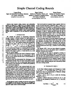
Fig. 2. Attainable channel regions for two parallel binary-input AWGN channels, as determined by the cutoff rate and the capacity limit, referring to a code rate of one-third bits per channel use. It is assumed that each bit is randomly and independently assigned to one of these channels with equal probability (i.e., α1 = α2 = 12 ).

In order to simplify the numerical computation of the capacity, one can express each integral in (10) as a sum of two integrals from 0 to ∞, and use the power series expansion of the logarithmic function; this gives an infinite power series with alternating signs. Using the Euler transform to expedite the convergence rate of these infinite sums, gives the following alternative expression:   2 βj ∞ k · ∆k a (j) X 1  2βe− 2 (−1) 0  , j = 1, . . . , J √ Cj = 1 − (11) − (2βj2 − 1)Q(βj ) + ln(2) 2k+1 2π k=0 where

µ µ ¶ ¶¾ k ½ (2k − 2m + 3)βj (−1)m k 1 − βj2 X √ erfcx ∆ a0 (j) , e 2 2 (k − m + 1)(k − m + 2) m 2 k

m=0

and

√ 2 erfcx(x) , 2ex Q( 2x)

(note that erfcx(x) ≈ √1π · x1 for large values of x). The infinite sum in (11) converges exponentially fast with k , and the summation of its first 30 terms gives very accurate results irrespectively of the value of βj .

6

³ ´ Eb Consider again the case of J = 2 parallel binary-input AWGN channels. Given the value of N , and the code 0 1 ³ ´ Eb rate R (in bits per channel use), (9) and (10) enable one to calculate the value of N for the second channel, 0 2 referring to the capacity limitation. To this end, one needs to set C in the LHS of (9) to the code rate R, and ³ ´ Eb find the resulting value of N0 which corresponds to the capacity limit. The boundary of the capacity region is 2

represented by the continuous curve in Fig. 2 for R = 31 bits per channel use; it is compared to the dashed curve in this figure which represents the boundary of the attainable channel region referring to the cutoff-rate limit (see Eq. (8)). C. Distance Properties of Ensembles of Turbo-Like Codes

In this paper, we exemplify our numerical results by considering several ensembles of binary linear codes. Due to the outstanding performance of turbo-like codes, our focus is mainly on such ensembles, where we also consider as a reference the ensemble of fully random block codes which achieves capacity under ML decoding. The other ensembles considered in this paper include turbo codes, repeat-accumulate codes and some recent variations. Bounds on the ML decoding error probability are often based on the distance properties of the considered codes or ensembles (see, e.g., [33] and references therein). The distance spectra and their asymptotic growth rates for various turbo-like ensembles were studied in the literature, e.g., for ensembles of uniformly interleaved repeataccumulate codes and variations [2], [9], [18], ensembles of uniformly interleaved turbo codes [4], [5], [25], [34], and ensembles of regular and irregular LDPC codes [6], [8], [14], [24]. In this subsection, we briefly present the distance properties of some turbo-like ensembles considered in this paper. Let us denote by [C(n)] an ensemble of codes of length n. We will also consider a sequence of ensembles [C(n1 )], [C(n2 )], . . . where all these ensembles possess a common rate R. For a given (n, k) linear code C , let ACh (or simply Ah ) denote the distance spectrum, i.e., the number of codewords of Hamming weight h. For a set of codes [C(n)], we define the average distance spectrum as X 1 [C(n)] ACh . (12) Ah , |[C(n)]| C∈[C(n)]

©1

ª Let Ψn , {δ : δ = nh for h = 1, . . . , n} = n , n2 , . . . , 1 denote the set of normalized distances, then the normalized exponent of the distance spectrum w.r.t. the block length is defined as [C(n)]

ln Ah ln ACh , r[C(n)] (δ) , . (13) n n The motivation for this definition lies in our interest to consider the asymptotic case where n → ∞. In this case we define the asymptotic exponent of the distance spectrum as rC (δ) ,

r[C] (δ) , lim r[C(n)] (δ) . n→∞

(14)

The input-output weight enumerator (IOWE) of a linear block code is given by a sequence {Aw,h } designating the number of codewords of Hamming weight h which are encoded by information bits whose Hamming weight is w. Referring to ensembles, one considers the average IOWE and distance spectrum over the ensemble. The distance spectrum and IOWE of linear block codes are useful for the analysis of the block and bit error probabilities, respectively, under ML decoding. As a reference to all ensembles, we will consider the ensemble of fully random block codes which is capacityachieving under ML decoding (or ’typical pairs’) decoding. The ensemble of fully random binary block codes: Consider the ensemble of binary random codes [RB], where the set [RB(n, R)] consists of all binary codes of length n and rate R. For this ensemble, the following well-known equalities hold: µ ¶ n −n(1−R) [RB(n,R)] 2 Ah = h ¡ ¢ ln nh [RB(n,R)] − (1 − R) ln 2 (15) r (δ) = n r[RB(R)] (δ) = H(δ) − (1 − R) ln 2

7

where H(x) , −x ln(x) − (1 − x) ln(1 − x) designates the binary entropy function to the natural base. Non-systematic repeat-accumulate codes: The ensemble of uniformly interleaved and non-systematic repeataccumulate (NSRA) codes [9] is defined as follows. The information block of length N is repeated q times by the encoder. The bits are then uniformly reordered by an interleaver of size qN , and, finally, encoded by a rate-1 differential encoder (accumulator), i.e., a truncated rate-1 recursive convolutional encoder with a transfer function (qN )! 1/(1 + D). The ensemble [NSRA(N, q)] is defined to be the set of (q!) N N ! RA different codes when considering the 1 different possible permutations of the interleaver. The (average) IOWE of the ensemble of uniformly interleaved RA codes RAq (N ) was originally derived in [9, Section 5], and it is given by ¡N ¢¡qN −h¢¡ h−1 ¢ NSRA(N,q)

Aw,h

=

d qw e−1 c b qw 2 ¡qN ¢ 2 qw

w

.

(16)

The average distance spectrum of the ensemble is therefore given by c) ¡N ¢¡qN −h¢¡ h−1 ¢ min(N,b 2h q lq m jq k X w e−1 d qw b qw c NSRA(N,q) 2 2 , ≤ h ≤ qN − Ah = ¡qN ¢ 2 2 qw w=1

§ ¨ NSRA(N,q) NSRA(N,q) where Ah = 0 for 1 ≤ h < 2q , and A0 = 1 since the all-zero vector is always a codeword of a linear code. The asymptotic exponent of the distance spectrum of this ensemble is given by (see [19]) r[NSRA(q)] (δ) ,

lim r[NSRA(N,q)] (δ) ¶ µ ¶ ½ µ ³ u ´¾ u 1 = max H(u) + (1 − δ)H + δH . − 1− q 2(1 − δ) 2δ 0≤u≤min(2δ,2−2δ) N →∞

(17)

0.3 NSRA codes Random codes

0.2

0.1

0

−0.1

−0.2

−0.3

−0.4

−0.5

0

0.1

0.2

0.3

0.4

0.5

0.6

0.7

0.8

0.9

1

Fig. 3. Plot of the asymptotic exponent of the distance spectra for the ensemble of fully random block codes, and the ensemble of uniformly interleaved and non-systematic repeat-accumulate (NSRA) codes of rate 31 bits per channel use. The curves are depicted as a function of the normalized Hamming weight (δ), and their calculations are based on (15) and (17).

The IOWEs and distance spectra of various ensembles of irregular repeat-accumulate (IRA) and accumulaterepeat-accumulate (ARA) codes are derived in [2], [18]. The reader is referred to Fig. 3, for a comparison between the asymptotic exponents (i.e., growth rates) of the distance spectra for the ensemble of fully random block codes and the ensemble of uniformly interleaved NSRA codes where both ensembles are assumed to be of rate one-third 1 There are (qN )! ways to place qN bits. However, permuting the q repetitions of any of the N information bits does not affect the result )! possible ways for the interleaving. Strictly speaking, by permuting the N information bits, the vector of the interleaving, so there are (qN (q!)N

space of the code does not change, which then yields that there are

(qN )! (q!)N N !

distinct RA codes of dimension k and number of repetitions q.

8

bit per channel use. One can observe from Fig. 3 that the two curves deviate considerably at low and high values of the normalized Hamming weight, while there is a good match between these two curves for intermediate values of the normalized Hamming weight. D. The DS2 Bound for a Single MBIOS Channel The bounding technique of Duman and Salehi [11], [12] originates from the 1965 Gallager bound [15] which states that the conditional ML decoding error probability Pe|m given that a codeword xm (of block length n) is transmitted is upper-bounded by  !λ ρ Ã 0 m X X ¡ ¢ pn (y|x )  λ, ρ ≥ 0 (18) pn y|xm  Pe|m ≤ m) p (y|x n 0 y m 6=m

where pn (y|x) designates the conditional pdf of the communication channel to obtain an n-length sequence y at the channel output, given the n-length input sequence x. Unfortunately, this upper bound is not calculable in terms of the distance spectrum of the code ensemble, except for the ensembles of fully random block codes and orthogonal codes transmitted over a memoryless channel, and the special case where ρ = 1, λ = 0.5 in which the bound reduces to the union-Bhattacharyya bound. With the intention of alleviating the difficulty of calculating the bound for specific codes and ensembles, we introduce the (m) function Ψn (y) which is an arbitrary probability tilting measure. This function may depend in general on the index R (m) m of the transmitted codeword [36], and is a non-negative function which satisfies the equality y Ψn (y) dy = 1. The upper bound in (18) can be rewritten in the following equivalent form:  ! ρ Ã m0 ) λ X X 1 ¡ ¢ p (y|x 1 n   (m) − ρ pn y|xm ρ λ, ρ ≥ 0. (19) Pe|m ≤ Ψ(m) n (y) Ψn (y) m) p (y|x n 0 y m 6=m

(m)

Recalling that Ψn

is a probability measure, we invoke Jensen’s inequality in (19) which gives  ! ρ Ã m0 ) λ X X p (y|x 1 1 n 1− ρ  , 0≤ρ≤1 Pe|m ≤  pn (y|xm ) ρ Ψ(m) n (y) m) λ≥0 p (y|x n 0 y

(20)

m 6=m

which is the DS2 bound. This expression can be simplified (see, e.g., [36]) for the case of a single memoryless channel where n Y pn (y|x) = p(yi |xi ). i=1

Let us consider probability tilting measures

(m) Ψn (y)

Ψ(m) n (y)

which can be factorized into the form =

n Y

ψ (m) (yi )

i=1

ψ (m)

recalling that the function may depend on the transmitted codeword xm . In this case, the bound in (20) is calculable in terms of the distance spectrum of the code, thus not requiring the fine details of the code structure. Let C be a binary linear block code whose length is n, and let its distance spectrum be given by {Ah }nh=0 . Consider the case where the transmission takes place over an MBIOS channel. By partitioning the code into subcodes of constant Hamming weights, let Ch be the set which includes all the codewords of C with Hamming weight h and the all-zero codeword. Note that this forms a partitioning of a linear code into subcodes which are in general non-linear. We apply the DS2 bound on the conditional ML decoding error probability (given the all-zero codeword is transmitted), and finally use the union bound w.r.t. the subcodes {Ch } in order to obtain an upper bound on the ML decoding error probability of the code C . Referring to the constant Hamming weight subcode Ch , the bound (20) gives à !n−h à !h  ρ  X  X 1−λρ 1 1 1 0≤ρ≤1 ψ(y)1− ρ p(y|0) ρ p(y|1)λ Pe|0 (h) ≤ (Ah )ρ . (21) ψ(y)1− ρ p(y|0) ρ λ≥0   y

y

9

Clearly, for an MBIOS channel with continuous output, the sums in (21) are replaced by integrals. In order to obtain the tightest bound within this form, the probability tilting measure ψ and the parameters λ and ρ are optimized. The optimization of ψ is based on calculus of variations, and is independent of the distance spectrum (this will be proved later also for the case of independent parallel MBIOS channels). Due to the symmetry of the channel and the linearity of the code C , the decoding error probability of C is independent of the transmitted codeword. Since the code C is the union of the subcodes {Ch }, the union bound provides an upper bound on the ML decoding error probability of C which is expressed as the sum of the conditional decoding error probabilities of the subcodes Ch given that the all-zero codeword is transmitted. Let dmin be the minimum distance of the code C , and R be the rate of the code C . Based on the linearity of the code, the geometry of the Voronoi regions (see [3]) gives the following expurgated union bound: n(1−R)

Pe ≤

X

h=dmin

Pe|0 (h).

(22)

For the bit error probability, one may partition a binary linear block code C into subcodes w.r.t. the Hamming weights of the information bits and the code bits. Let Cw,h designate the subcode which includes the all-zero codeword and all the codeowrds of C whose Hamming weight is h and whose information bits have Hamming weight w. An upper bound on the bit error probability of the code C is performed by calculating the DS2 upper bound on the conditional bit error probability for each subcode Cw,h (given that the all-zero codeword is transmitted), and applying the union bound over all these subcodes. Note that the number of these subcodes is at most quadratic in the block length of the code, so taking the union bound w.r.t. these subcodes does not affect the asymptotic tightness of the overall bound. Let {Aw,h } designate the IOWE of the code C whose block length and dimension are equal to n and k , respectively. The conditional DS2 bound on the bit error probability was demonstrated in [32], [33] to be identical to the DS2 bound on the block error probability, except that the distance spectrum of the code k X Aw,h , h = 0, . . . , n (23) Ah = w=0

appearing in the RHS of (21) is replaced by A0h ,

k ³ ´ X w

w=0

k

Aw,h ,

h = 0, . . . , n.

(24)

Since A0h ≤ Ah then, as expected, the upper bound on the bit error probability is smaller than the upper bound on the block error probability. Finally, note that the DS2 bound is also applicable to ensembles of linear codes. To this end, one simply needs to replace the distance spectrum or the IOWE of a code by the average quantities over this ensemble. This follows easily by invoking Jensen’s inequality to the RHS of (21) which yields that E[(Ah )ρ ] ≤ (E[Ah ])ρ for 0 ≤ ρ ≤ 1. The DS2 bound for a single channel is discussed in further details in [11], [32], [36] and the tutorial paper [33, Chapter 4]. III. G ENERALIZED DS2 B OUNDS

FOR I NDEPENDENT

PARALLEL C HANNELS

In this section, we generalize the DS2 bound to independent parallel MBIOS channels, and optimize the probability tilting measures in the generalized bound to obtain the tightest bound within this form. We will discuss two possible ways of generalizing the bound. These two versions of the bound are obtained via different way of looking on the set of parallel channels and their tightness is compared. A. Generalizing the DS2 bound to Parallel Channels: First Approach 1) Derivation of the new bound in the first approach: Let us assume that the communication takes place over J statistically independent parallel channels where each one of the individual channels is memoryless binary-input output-symmetric (MBIOS) with antipodal signaling, i.e., p(y|x = 1) = p(−y|x = −1). The essence of the approach discussed in this section is to start by considering the case of a specific channel assignment; the calculation then

10

proceeds by averaging the bound over all possible assignments. For a specific channel assignment, the assumption that all J channels are independent and MBIOS means that we factor the transition probability as J Y ¡ ¢ Y (m) pn y|xm = p(yi |xi ; j)

(25)

j=1 i∈I(j)

which we can plug into (20) to get a DS2 bound suitable for the case of parallel channels. In order to get a bound which depends on one-dimensional sums (or one-dimensional integrals), we impose a restriction on the tilting (m) measure Ψn (·) in (20) so that it can be expressed as a J -fold product of one-dimensional probability tilting measures, i.e., J Y Y = Ψ(m) (y) ψ (m) (yi ; j). (26) n j=1 i∈I(j)

Considering a binary linear blockPcode C , the conditional decoding error probability does not depend on the M −1 1 transmitted codeword, so Pe , M m=0 Pe|m = Pe|0 where w.o.l.o.g., one can assume that the all-zero vector is the transmitted codeword. The channel mapper for the J independent parallel channels is assumed to transmit the bits whose indices are included in the subset I(j) over the j -th channel where the subsets {I(j)} constitute a disjoint partitioning of the set of indices {1, 2, . . . , n}. Following the notation in [23], let Ah1 ,h2 ,...,hJ designate the split weight enumerator of the binary linear block code, defined as the number of codewords of Hamming weight hj within the J disjoint subsets I(j) for j = 1 . . . J . By substituting (25) and (26) in (20), we obtain Pe = Pe|0   µ ¶λ ρ |I(J)| J |I(1)| X X X Y Y 1 1 p(yi |xi ; j) ≤ ... Ah1 ,h2 ,...,hJ ψ(yi ; j)1− ρ p(yi |0; j) ρ   p(yi |0; j) y =

=

h1 =0

hJ =0

j=1 i∈I(j)

 |I(1)| X

|I(J)|

J Y Y X

...

X

Ah1 ,h2 ,...,hJ



h1 =0

hJ =0

j=1 i∈I(j) yi

 |I(1)| X

|I(J)|



h1 =0

à J X Y

...

X

Ah1 ,h2 ,...,hJ

hJ =0

j=1

à J X Y

j=1

y

1

1

ψ(yi ; j)1− ρ p(yi |0; j) ρ

ψ(y; j)

1− ρ1

p(y|0; j)

1−λρ ρ

1

ψ(y; j)1− ρ p(y|0; j) ρ



p(yi |xi ; j) p(yi |0; j) λ

p(y|1; j)

y

!|I(j)|−hj ρ  1

µ

,

!hj

0≤ρ≤1 . λ≥0

 ¶λ ρ 

(27)

We note that the bound in (27) is valid for a specific assignment of bits to the parallel channels. For structured codes or ensembles, the split weight enumerator is in general not available when considering specific assignments. As a result of this, we continue the derivation by using the random assignment approach. Let us designate nj , |I(j)| to be the cardinality of the set I(j), so E[nj ] = αj n is the expected number of bits assigned to channel no. j (where j = 1, 2, . . . , J). Averaging (27) with respect to all possible channel assignments, we get the following bound on

11

the average ML decoding error probability:  Ã !hj nJ n1 J X X Y X 1−λρ 1 Ah1 ,h2 ,...,hJ ψ(y; j)1− ρ p(y|0; j) ρ p(y|1; j)λ ... Pe ≤ E  y j=1 hJ =0 h1 =0 !nj −hj ρ Ã J  X Y 1 1 ψ(y; j)1− ρ p(y|0; j) ρ  y j=1  Ã !hj nJ n1 J X Y X X X 1−λρ 1− ρ1 λ ψ(y; j) Ah1 ,h2 ,...,hJ ... = p(y|0; j) ρ p(y|1; j)  y Pnj ≥0 j nj =n

h1 =0

hJ =0

j=1

à J X Y

!nj −hj ρ  1

1

ψ(y; j)1− ρ p(y|0; j) ρ

PN (n)

(28)



y

j=1

where PN (n) designates the probability distribution of the discrete random vector N , (n1 , . . . , nJ ). Applying Jensen’s inequality to the RHS of (28) and changing the order of summation give ( n X X X Pe ≤ Ah1 ,h2 ,...,hJ PN (n) Pnj ≥0 h=0 h1 ≤n1 ,...,hJ ≤nJ h1 +...+hJ =h nj =n

à J X Y

j=1

p(y|0; j)

1−λρ ρ

λ

p(y|1; j)

y

à J X Y

j=1

ψ(y; j)

1− ρ1

ψ(y; j)

1− ρ1

p(y|0; j)

y

1 ρ

!nj −hj )ρ

,

!hj 0≤ρ≤1 . λ≥0

(29)

to the bits transmitted over Let the vector H = (h1 , . . . , hJ ) be the vector of partial Hamming weights referringP each channel (nj bits are transmitted over channel no. j , so 0 ≤ hj ≤ nj ). Clearly, Jj=1 hj = h is the overall Hamming weight of a codeword in C . Due to the random assignment of the code bits to the parallel channels, we get ¶ µ n PN (n) = α1n1 α2n2 . . . αJnJ n1 , n2 , . . . , nJ ¡ h ¢¡ ¢ n−h PH|N (h|n) =

h1 ,...,hJ

Ah1 ,h2 ,...,hJ PN (n)

¡

n1 −h1 ,...,nJ −hJ ¢ n n1 ,...,nJ

= Ah PH|N (h|n) PN (n) µ ¶µ ¶ h n−h nJ n1 n2 = Ah α1 α2 . . . αJ h1 , . . . , hJ n1 − h1 , . . . , nJ − hJ

(30)

12

and the substitution of (30) in (29) gives ( n X X Ah Pe ≤ Pnj ≥0 h=0 nj =n

X

h1 ≤n1 ,...,hJ ≤nJ h1 +...+hJ =h

µ

h h1 , h2 , . . . , hJ

¶

¶ n−h n1 − h1 , n2 − h2 , . . . , nJ − hJ Ã !h j J X Y 1−λρ 1− ρ1 λ ψ(y; j) αj p(y|0; j) ρ p(y|1; j)

µ

y

j=1 J Y

j=1

Ã

αj

X

ψ(y; j)

1− ρ1

p(y|0; j)

1 ρ

y

!nj −hj )ρ

.

Let kj , nj − hj for j = 1, 2, . . . , J , then by changing the order of summation we obtain   Ã !hj  µ ¶Y n J X X X 1−λρ h 1− ρ1 λ Ah ψ(y; j) αj Pe ≤ p(y|0; j) ρ p(y|1; j)  h1 , h2 , . . . , hJ  y j=1 h1 ,...,hJ ≥0 h=0 h1 +...+hJ =h

X

k1 ,...,kJ ≥0 k1 +...+kJ =n−h

Since

PJ

j=1 hj

= h and Pe

µ

n−h k1 , k2 , . . . , kJ

¶Y J

j=1

Ã

αj

X

1

ψ(y; j)1− ρ p(y|0; j) ρ

y

PJ

j=1 kj = n − h, the use of the multinomial formula gives   h  J n X X X 1−λρ 1 Ah  ≤ ψ(y; j)1− ρ p(y|0; j) ρ p(y|1; j)λ  αj  h=0 y j=1

n−h ρ   X 1 1− ρ1   ρ ψ(y; j) αj p(y|0; j)   y j=1 

J X

ρ !k j    1

0≤ρ≤1 P λ≥0 y ψ(y; j) = 1 j = 1...J

  

(31)

which forms a possible generalization of the DS2 bound for independent parallel channels when averaging over all possible channel assignments. This result can be applied to specific codes as well as to structured ensembles for which the average distance spectrum Ah is known. In this case, the average ML decoding error probability Pe is obtained by replacing Ah in (31) with the average distance spectrum Ah (this can be verified by noting that the function f (t) = tρ is concave for 0 ≤ ρ ≤ 1 and by invoking Jensen’s inequality in (31)). In the continuation of this section, we propose an equivalent version of the generalized DS2 bound for parallel channels where this equivalence follows the lines in [33], [36]. Rather than relying on a probability (i.e., normalized) tilting measure, the bound will be expressed in terms of an un-normalized tilting measure which is an arbitrary non-negative function. This version will be helpful later for the discussion on the connection between the DS2 bound and the 1961 Gallager bound for parallel channels, and also for the derivation of some particular cases of (m) the DS2 bound. We begin by expressing the DS2 bound using the un-normalized tilting measure Gn which is (m) related to Ψn by (m) Gn (y)pn (y|xm ) (m) . (32) Ψn (y) = X 0 0 m G(m) n (y )pn (y |x ) y0

13

Substituting (32) in (20) gives Pe|m ≤

 X X

Ã

1− ρ1

0

pn (y|xm ) pn (y|xm )

G(m) pn (y|xm ) n (y)  0 m 6=m y 1−ρ  X 0≤ρ≤1 m   , . G(m) n (y)pn (y|x ) λ≥0

!λ ρ  

y

(m)

As before, we assume that Gn

can be factored in the product form G(m) n (y) =

J Y Y

g(yi ; j).

j=1 i∈I(j)

Following the algebraic steps in (27)-(31) and averaging as before also over all the codebooks of the ensemble, we obtain the following upper bound on the ML decoding error probability:   Ã ! J n X X X 1 1− 1−λ λ Ah  αj Pe = Pe|0 ≤ g(y; j) ρ p(y|0; j) p(y|1; j)  y j=1 h=0 Ã ! Ã ! 1−ρ h  J ρ X X X 1 1−   αj g(y; j) ρ p(y|0; j) g(y; j)p(y|0; j) y

à X y

j=1

y

 ! 1−ρ n−h ρ ρ  0≤ρ≤1  , . g(y; j)p(y|0; j) λ≥0  

(33)

Note that the generalized DS2 bound as derived in this subsection is applied to the whole code (i.e., the optimization of the tilting measures refers to the whole code and is performed only once for each of the J channels). In the next subsection, we consider the partitioning of the code to constant Hamming weight subcodes, and then apply the union bound. For every such subcode, we rely on the conditional DS2 bound (given the all-zero codeword is transmitted), and optimize the J tilting measures; this optimization is performed for each of the subcodes separately. The total number of subcodes does not exceed the block length of the code (or ensemble), and hence the use of the union bound in this case does not degrade the related error exponent of the overall bound; moreover, the optimized tilting measures are tailored for each of the constant-Hamming weight subcodes, a process which can only improve the exponential behavior of the resulting bound. 2) Optimization of the Tilting Measures: In the following, we find optimized tilting measures {ψ(·; j)}Jj=1 which minimize the DS2 bound (31). The following calculation is a possible generalization of the analysis in [36] for a single channel to the considered case of an arbitrary number (J) of independent parallel MBIOS channels. Let C be a binary linear block code of length n. Following the derivation in [23], [36], we partition the code C to constant Hamming weight subcodes {Ch }nh=0 , where Ch includes all the codewords of weight h (h = 0, . . . , n) as well as the all-zero codeword. Let Pe|0 (h) denote the conditional block error probability of the subcode Ch under ML decoding, given that the all-zero codeword is transmitted. Based on the union bound, we get Pe ≤

n X h=0

Pe|0 (h).

(34)

As the code C is linear, Pe|0 (h) = 0 for h = 0, 1, . . . , dmin − 1 where dmin denotes the minimum distance of the code C . The generalization of the DS2 bound in (31) gives the following upper bound on the conditional error

14

probability of the subcode Ch :

 δ  J  X X 1−λρ 1 Pe|0 (h) ≤ (Ah )ρ  ψ(y; j)1− ρ p(y|0; j) ρ p(y|1; j)λ  αj   j=1 y 1−δ nρ   J  X X 1 h 0≤ρ≤1 1− ρ1   ρ p(y|0; j) δ, . , ψ(y; j) αj λ≥0  n  y j=1

(35)

Note that in this case, the set of probability tilting measures {ψ(·; j)}Jj=1 may also depend on the Hamming weight (h) of the subcode (or equivalently on δ ). This is the result of performing the optimization on every individual constant-Hamming subcode instead of the whole code. This generalization of the DS2 bound can be written equivalently in the exponential form DS21 h Pe|0 (h) ≤ e−nEδ (λ,ρ,J,{αj }) , 0 ≤ ρ ≤ 1, λ ≥ 0, δ , . (36) n where   J X X 1−λρ 1 E DS21 (λ, ρ, J, {αj }) , −ρr[C] (δ) − ρδ ln  ψ(y; j)1− ρ p(y|0; j) ρ p(y|1; j)λ  αj δ

y

j=1



−ρ(1 − δ) ln 

J X j=1

αj

X y

1

1



ψ(y; j)1− ρ p(y|0; j) ρ 

and r[C] (δ) designates the normalized exponent of the distance spectrum as in (14). Let µ ¶ 1 1 p(y|1; j) λ ρ ρ g1 (y; j) , p(y|0; j) , g2 (y; j) , p(y|0; j) p(y|0; j)

(37)

(38)

then, for a given pair of λ and ρ (where λ ≥ 0 and 0 ≤ ρ ≤ 1), we need to minimize     J J X X X X 1 1 δ ln  ψ(y; j)1− ρ g1 (y; j) αj ψ(y; j)1− ρ g2 (y; j) + (1 − δ) ln  αj j=1

y

j=1

y

over the set of non-negative functions ψ(· ; j) satisfying the constraints X ψ(y; j) = 1, j = 1 . . . J.

(39)

y

To this end, calculus of variations provides the following set of equations: Ã αj (1 − δ)(1 − ρ1 )g1 (y; j) 1 −ρ ψ(y; j) P PJ 1− ρ1 g1 (y; j) y j=1 αj ψ(y; j) ! αj δ(1 − ρ1 )g2 (y; j) + ξj = 0, +P P 1− ρ1 J g (y; j) α ψ(y; j) 2 j y j=1

j = 1, . . . , J

(40)

where ξj is a Lagrange multiplier. The solution of (40) is given in the following implicit form: ¡ ¢ρ ψ(y; j) = k1,j g1 (y; j) + k2,j g2 (y; j) , k1,j , k2,j ≥ 0, j = 1, . . . , J

where

J X X

k2,j δ j=1 y∈Y = J X k1,j 1−δX j=1 y∈Y

1

αj ψ(y; j)1− ρ g1 (y; j) . αj ψ(y; j)

1− ρ1

g2 (y; j)

(41)

15 ρ 2,j in the RHS of (41) is independent of j . Thus, the substitution βj , k1,j gives that the We note that k , kk1,j optimal tilting measures can be expressed as ¡ ¢ρ ψ(y; j) = βj g1 (y; j) + kg2 (y; j) " µ ¶ #ρ p(y|1; j) λ = βj p(y|0; j) 1 + k y ∈ Y j = 1, . . . , J. (42) p(y|0; j)

By plugging (38) into (41) we obtain   " µ ¶λ #ρ−1  J X X 1− ρ1 p(y|1; j) p(y|0; j) 1 + k α β  j j  p(y|0; j) j=1 y∈Y δ   k= µ µ ¶λ " ¶λ #ρ−1  1−δX J X 1 1− p(y|1; j) p(y|1; j) 1+k αj βj ρ p(y|0; j)   p(y|0; j) p(y|0; j)

(43)

j=1 y∈Y

and from (38) and (39), βj which is the appropriate factor normalizing the probability tilting measure ψ(·; j) in (42) is given by " Ã µ ¶ !ρ #−1 X p(y|1; j) λ βj = p(y|0; j) 1 + k , j = 1, . . . , J. (44) p(y|0; j) y Note that the implicit equation for k in (43) and the normalization coefficients in (44) provide a possible generalization of the results derived in [32, Appendix A] (where k is replaced there by α). The point here is that the 2,j in (41) is independent of j (where j ∈ {1, 2, . . . , J}), a property which significantly simplifies the value of kk1,j optimization process of the J tilting measures, and leads to the result in (42). For the numerical calculation of the bound in (35) as a function of the normalized Hamming weight δ , nh , and for a fixed pair of λ and ρ (where λ ≥ 0 and 0 ≤ ρ ≤ 1), we find the optimized tilting measures in (42) by first assuming an initial vector β (0) = (β1 , . . . , βJ ) and then iterating between (43) and (44) until we get a fixed point for these equations. For a fixed δ , we need to optimize numerically the bound in (36) w.r.t. the two parameters λ and ρ. B. Generalizing the DS2 bound to Parallel Channels: Second Approach 1) Derivation of the new bound in a second approach: In this section we show a second way of generalizing the DS2 bound for independent parallel MBIOS channels. We begin by suggesting a system model equivalent to the one presented in Sec. II-A which we term the channel side information at the receiver (CSIR) model. Rather than viewing the set of component channels as parallel channels, we consider j (where 1 ≤ j ≤ J ) to be the internal state of a state-dependent channel p(y|x; j) to which x is the input and y is the output. As in the parallel-channel model shown in Fig. 1, j is chosen at random for each transmitted symbol according to the a-priori probability distribution {αj } from the finite alphabet {1, 2, . . . , J}. Therefore, these two channel models are identical, except that we have to include the receiver’s perfect knowledge of the channel state in the CSIR model. This is easily accomplished by viewing the internal state j as part of the output of the channel, i.e., the output is the pair b , (y, j); the transition probability of this channel is thus denoted by pB (b|x). Since the channel and channel mapper both operate in a memoryless manner, the CSIR channel model is also memoryless. Finally, the transition probability pB (b|x) satisfies the relation pB (b|x) = αj p(y|x; j) (45) because the channel state is independent of the input. If we define −b , (−y, j), then we obtain from (45) and the symmetry of the transition probabilities p(y|x; j) that pB (b|x) = pB (−b| − x); thus, the CSIR model is also symmetric. In summary, the parallel-channel model presented in Sec. II-A is equivalent to an MBIOS channel with transition probability given in (45). We may thus use the DS2 bounding technique directly on the CSIR model; using this approach, the need to average over all channel mappings is circumvented.

16

Following this approach, we set the channel output to be b = (y, j) and substitute (45) into (21) to get the upper bound  h J 1 X X 1−λρ 1 Pe ≤ (Ah )ρ  αjρ ψ(y; j)1− ρ p(y|0; j) ρ p(y|1; j)λ  y

j=1

 

J X

1 ρ

αj

X

ψ(y; j)

1− ρ1

y

j=1

1 ρ

n−h

p(y|0; j) 

0≤ρ≤1 P λ≥0 y,j ψ(y; j) = 1

(46)

As in the first approach (see (33)), this bound may also be expressed in terms of an un-normalized tilting measure, rather than a normalized (probability) measure. We will use this version later when we discuss special cases of this bound. The DS2 bound for parallel channels obtained using the second approach which is expressed using the un-normalized tilting measure is as follows:  n(1−ρ) J X X Pe ≤ (Ah )ρ  g(y; j)p(y|0; j) αj y

j=1

 !hρ Ã J X X 1  αj g(y; j)1− ρ p(y|0; j)1−λ p(y|1; j)λ  y

j=1

 !(n−h)ρ Ã J X X 1 0≤ρ≤1  . , αj g(y; j)1− ρ p(y|0; j)  λ≥0

(47)

y

j=1

We turn our attention to the derivation of optimized tilting measures for the generalized DS2 bound obtained using the second approach. 2) Optimization of the Tilting Measures: The optimization of tilting measures for the generalized DS2 bound in (46) obtained using the perfect CSIR model relies on this optimization for MBIOS channels. As in the first approach, the bound for a specific constant Hamming-weight subcode is expressed in exponential form DS22

Pe|0 (h) ≤ e−nEδ

(λ,ρ,J,{αj })

,

0 ≤ ρ ≤ 1,

λ ≥ 0,

δ,

h n

(48)

where   J 1 X X 1−λρ 1 EδDS22 (λ, ρ, J, {αj }) , −ρr[C] (δ) − ρδ ln  αjρ ψ(y; j)1− ρ p(y|0; j) ρ p(y|1; j)λ  y

j=1



−ρ(1 − δ) ln 

J X j=1

1 ρ

αj

X y

ψ(y; j)

1− ρ1

1 ρ



p(y|0; j)  .

(49)

The optimized tilting measure should be chosen so as to maximize the exponent in (49). Since the perfect CSIR model is equivalent to an MBIOS channel, we can use the results of Sec. III-A.2 with J = 1; by substituting the transition probability from (45) into (42), we obtain that the optimal form of the tilting measure is given by à ¶ !ρ µ p(y|1; j) λ (50) ψ(y; j) = βαj p(y|0; j) 1 + k p(y|0; j) where k is a parameter to be optimized and β is a normalizing constant given by   à ¶λ !ρ −1 µ X p(y|1; j)  β= αj p(y|0; j) 1 + k p(y|0; j) y,j

(51)

17

C. Comparison Between the Two Generalized DS2 Bounds for Parallel Channels Let us examine the two generalizations of the DS2 bound proposed in Sections III-A and III-B for the purpose of comparison. To this end, for constant weight subcodes of Hamming weight h (including the all-zero codeword), we write out the explicit expressions for the two bounds, including the optimal form of the tilting measures. By substituting (42) with the optimal value of k in (43), the bound in (31) obtained by the first approach reads    µ µ ¶λ Ã ¶λ !ρ−1 h J  X 1 X 1− p(y|1; j) p(y|1; j) (1)  Pe|0 (h) ≤ (Ah )ρ  βj ρ p(y|0; j) αj 1 + kopt  p(y|0; j) p(y|0; j)  j=1 y   Ã !ρ−1 n−h ρ µ ¶ J λ  X X 1− 1 (1) p(y|1; j)   . (52) βj ρ p(y|0; j) 1 + kopt αj  p(y|0; j)  y j=1 In the same way, substituting (50) in (46) gives the bound obtained by using the second approach    µ µ ¶λ Ã ¶λ !ρ−1 h J  X X 1 p(y|1; j) p(y|1; j) (2)  1 + kopt β 1− ρ p(y|0; j) Pe|0 (h) ≤ (Ah )ρ  αj  p(y|0; j) p(y|0; j)  j=1 y   Ã !ρ−1 n−h ρ µ ¶ J λ  X X 1− 1 (2) p(y|1; j)   β ρ p(y|0; j) 1 + kopt αj .  p(y|0; j)  y j=1

(53)

From these expressions one cannot conclusively deduce the superiority of one of the bounds over the other in general. However, in the random coding setting, it can be shown that the DS2 bound in Section III-B is tighter than the one in Section III-A. To this end, we show that the former bound attains the random coding exponent [15] while the latter does not. The random coding exponent which corresponds to the MBIOS channel given by the perfect CSIR model, from which the second version in Section III-B is derived, gives the relation Pe ≤ 2−n(E0 (ρ)−ρR)

0≤ρ≤1

(54)

where E0 (ρ) = − log2

à X µ1 b



= − log2 

J X j=1

2

αj

pB (b|0)

X µ1 y

1 1+ρ

1 1 + pB (b|1) 1+ρ 2

¶1+ρ !

1 1 1 p(y|0; j) 1+ρ + p(y|1; j) 1+ρ 2 2

¶1+ρ

 

(55)

We now turn to find the random coding exponent which stems from the use of the bound in Section III-B. We start with the bound in (47) which is expressed in terms of the un-normalized tilting measure. Consider the following choice for the un-normalized tilting measure · ¸ρ ρ 1 1 1 1 1+ρ 1+ρ g(y; j) = p(y|0; j) p(y|0; j)− 1+ρ , j = 1, 2, . . . , J + p(y|1; j) (56) 2 2 and the distance spectrum of the ensemble of random binary block codes of length n and rate R, given by µ ¶ −n(1−R) n Ah = 2 , h = 0, 1, . . . , n. h 1 gives the bound Substituting (56) and (57) into (33) and setting λ = 1+ρ   ¸1+ρ n J X X ·1 1 1 1 Pe ≤ 2nRρ p(y|0; j) 1+ρ + p(y|1; j) 1+ρ αj   2 2 y j=1

(57)

(58)

18

which coincides with the random coding bound in (54)-(55). By substituting the tilting measure (56) in the bound in Section III-A (see (31)) we get the following error exponent, which appears instead of E0 (ρ) in (55)   Ã !1+ρ  ρ1 ρ J X X1 1 1 1 ˜0 (ρ) = − log2    E αj  p(y|0; j) 1+ρ + p(y|1; j) 1+ρ   . 2 2 y j=1

˜0 (ρ) ≤ E0 (ρ), and we therefore Using Jensen’s inequality and the fact that 0 ≤ ρ ≤ 1, it is easy to show that E conclude that the bound from Section III-B is tighter than the one in Section III-A in the random coding setting. Discussion. When comparing the two versions of the bound, it should be noted that the two optimized forms of tilting measures as given in (42) and (50) are not identical. While these two forms of tilting measures exhibit the same functional behavior, the normalization conditions are slightly different, with J normalizing constants in the first version of the bound (see (44)) and one constant (see (51)) in the second version. This hints that either of these bounds in (52) and (53) is not uniformly tighter than the other for general codes or ensembles; this was also verified numerically by comparing the two bounds for some code ensembles. For random codes, we note that the tightness of the first version is hindered by the use of Jensen’s inequality which is applied in the process of averaging over all possible channel assignments (see the move from (28) to (29)). This application of Jensen’s inequality does not appear in the derivation of the second version of the DS2 bound, and may be the seed of the pitfall of the first version, when applied for random codes.

D. Statement of the Main Result Derived in Section III The analysis in this section leads to the following theorem: Theorem 1 (Generalized DS2 bounds for independent parallel MBIOS channels): Consider the transmission of binary linear block codes (or ensembles) over a set of J independent parallel MBIOS channels. Let the pdf of the j th MBIOS channel be given by p(·|0; j) where due to the symmetry of the binary-input channels p(y|0; j) = p(−y|1; j). Assume that the coded bits are randomly and independently assigned to these channels, where each bit is transmitted over one of the J MBIOS channels. Let αj be the a-priori probability of transmitting a bit over the j th channel PJ (j = 1, 2, . . . , J ), so that αj ≥ 0 and j=1 αj = 1. By partitioning the code into constant Hamming-weight subcodes, Eqs. (35) and (46) provide two possible upper bounds on the conditional ML decoding error probability for each of these subcodes, given that the all-zero codeword is transmitted, and (34) forms an upper bound on the block error probability of the whole code (or ensemble). For the bound in (35), the optimized set of probability tilting measures {ψ(·; j)}Jj=1 which attains the minimal value of the conditional upper bound is given by the set of equations in (42); for the bound in (46), the optimal tilting measure is given in (50). IV. G ENERALIZATION

1961 G ALLAGER B OUND FOR PARALLEL C HANNELS AND I TS C ONNECTION TO THE G ENERALIZED DS2 B OUND The 1961 Gallager bound for a single MBIOS channel was derived in [14], and a generalization of the bound for parallel MBIOS channels was proposed by Liu et al. [23]. In the following, we outline the derivation in [23] which serves as a preliminary step towards the discussion of its relation to the two versions of the generalized DS2 bound from Section III. In this section, we optimize the probability tilting measures which are related to the 1961 Gallager bound for J independent parallel channels in order to get the tightest bound within this form (hence, the optimization is carried w.r.t. J probability tilting measures). This optimization differs from the discussion in [23] where the authors choose some simple and sub-optimal tilting measures. By doing so, the authors in [23] derive bounds which are easier for numerical calculation, but the tightness of these bounds is loosened as compared to the improved bound which relies on the calculation of the J optimized tilting measures (this will be exemplified in Section VII for turbo-like ensembles). OF THE

A. Presentation of the Bound [23] Consider a binary linear block code C . Let xm be the transmitted codeword and define the tilted ML metric à (m) ! (y) f 0 n Dm (xm , y) , ln (59) pn (y|xm0 )

19 (m)

0

where fn (y) is an arbitrary function which is positive if there exists m0 6= m such that pn (y|xm ) is positive. If the code is ML decoded, an error occurs if for some m0 6= m 0

Dm (xm , y) ≤ Dm (xm , y) .

As noted in [36], Dm (·, ·) is in general not computable at the receiver. It is used here as a conceptual tool to evaluate the upper bound on the ML decoding error probability. The received set Y n is expressed as a union of two disjoint subsets Y n = Ygn ∪ Ybn ª © Ygn , y ∈ Y n : Dm (xm , y) ≤ nd © ª Ybn , y ∈ Y n : Dm (xm , y) > nd

where d is an arbitrary real number. The conditional ML decoding error probability can be expressed as the sum of two terms Pe|m = Prob(error, y ∈ Ybn ) + Prob(error, y ∈ Ygn ) which is upper bounded by Pe|m ≤ Prob(y ∈ Ybn ) + Prob(error, y ∈ Ygn ) .

(60)

We use separate bounding techniques for the two terms in (60). Applying the Chernoff bound on the first term gives ¡ ¢ (61) P1 , Prob(y ∈ Ybn ) ≤ E esW , s ≥ 0 where

W , ln

Ã

(m)

fn (y) pn (y|xm )

!

− nd .

(62)

Using a combination of the union and Chernoff bounds for the second term in the RHS of (60) gives P2 , Prob(error, y ∈ Ygn ) ³ ´ 0 = Prob Dm (xm , y) ≤ Dm (xm , y) for some m0 6= m, y ∈ Ygn ³ ´ X 0 Prob Dm (xm , y) ≤ Dm (xm , y), Dm (xm , y) ≤ nd ≤ m0 6=m

≤

X

E (exp(tUm0 + rW )) ,

m0 6=m

t, r ≤ 0

(63)

where, based on (59),

¶ pn (y|xm ) Um0 = Dm (x , y) − Dm (x , y) = ln . (64) pn (y|xm0 ) Consider a codeword of a binary linear block code C which is transmitted over J parallel MBIOS channels. Since the conditional error probability under ML decoding does not depend on the transmitted codeword, one can assume without loss of generality that the all-zero codeword is transmitted. As in Section III-A, we impose on the function (m) fn (y) the restriction that it can be expressed in the product form m0

fn(m) (y)

m

=

J Y Y

j=1 i∈I(J)

µ

f (yi ; j) .

(65)

20

For the continuation of the derivation, it is assumed that the functions f (·; j) are even, i.e., f (y; j) = f (−y; j) for all y ∈ Y . Plugging (25), (62), (64) and (65) into (61) and (63) we get   J  X Y Y µ f (yi ; j) ¶s P1 ≤ p(yi |0; j) e−nsd   p(yi |0; j) y j=1 i∈I(j)  nj  J  X  Y  = p(y|0; j)1−s f (y; j)s  e−nsd s ≥ 0 (66)   j=1 y∈Y ( !t ) Ã J Y µ f (yi ; j) ¶r X X Y p(yi |0; j) e−nrd p(yi |0; j) P2 ≤ (m0 ) p(y |0; j) i p(yi |xi ; j) y m0 6=m j=1 i∈I(j)    µ ¶ t hj n1 nJ  J  X Y X X p(y|0; j)   p(y|0; j)1−r f (y; j)r Ah1 ,...,hJ = ...  p(y|1; j) j=1 y∈Y h1 =0 hJ =0  nj −hj    J  Y X 1−r r  e−nrd , t, r ≤ 0 (67) p(y|0; j) f (y; j)    j=1 y∈Y

where as before, we use the notation nj , |I(j)|. Optimizing the parameter t gives the value in [14, Eq. (3.27)] t=

r−1 . 2

(68)

Let us define X

G(r; j) ,

p(y|0; j)1−r f (y; j)r

(69)

y

X

Z(r; j) ,

[p(y|0; j)p(y|1; j)]

1−r 2

f (y; j)r .

(70)

y

Substituting (68) into (67), combining the bounds on P1 and P2 in (66) and (67), and finally averaging over all possible channel assignments, we obtain  Pe

n X  ≤ E

X

Ah1 ,...,hJ

h=1 0≤h P j ≤nj hj =h

+

=

Pnj ≥0 nj =n

J Y

X



[G(s; j)]nj e−nsd  Ah1 ,...,hJ

  h=1 0≤h P j ≤nj

+

J Y

nj −nsd

J Y

[Z(r; j)]hj [G(r; j)]nj −hj e−nrd

j=1

hj =h

[G(s; j)] e

j=1

[Z(r; j)]hj [G(r; j)]nj −hj e−nrd

j=1

j=1

  n X X 

J Y

  

PN (n)

,

r≤0 s≥0 . −∞ < d < ∞

(71)

21

Following the same procedure of averaging the bound over all possible assignments as in (30) and (31), we obtain   h  n−h   J n  J   X X X     Ah αj Z(r; j) Pe ≤ αj G(r; j) e−nrd    j=1 j=1 h=1   n J X  + αj G(s; j) e−nsd . (72) j=1

Finally, we optimize the bound in (72) over the parameter d which gives  n(1−ρ)  h  n−h ρ    J n J J X  X  X X Pe ≤ 2H(ρ) Ah  αj Z(r; j)  αj G(r; j) αj G(s; j)    h=1   j=1 j=1 j=1 where r ≤ 0, s ≥ 0, and

(73)

s , 0≤ρ≤1. (74) s−r The bound in (73), originally derived in [23], is a natural generalization of the 1961 Gallager bound for parallel channels. ρ,

B. Connection to the Generalizations of the DS2 Bound In this section we revisit the relations that exist between the DS2 bound and the 1961 Gallager bound, this time for the case of independent parallel channels. We will compare the 1961 Gallager bound with both versions of the DS2 bound presented in Sec. III. For the case of a single MBIOS channel, it was shown [10], [33], [36] that the DS2 bound is tighter than the 1961 Gallager bound. This result easily extends to parallel channels, for the case of the second version of the DS2 bound which was derived in Sec. III-B using the perfect CSIR channel model. Under this model, the parallel-channel is expressed as a single MBIOS with output defined as the pair b = (y, j). The results in [10], [33], [36] therefore apply directly to the CSIR model and can be used to show that the DS2 bound in (46) is tighter than the 1961 Gallager bound (73). In this respect, the DS2 bound from Section III-A exhibits a slightly different behavior. In the remainder of this section, we provide analysis linking this bound with the 1961 Gallager bound. In what follows, we will see how a variation in the derivation of the Gallager bound leads to a form of the DS2 bound from Section III-A, up to a factor which varies between 1 and 2. To this end, we start from the point in the last section where the combination of the bounds in (66) and (67) is obtained. Rather than continuing as in the last section, we first optimize over the parameter d in the sum of the bounds on P1 and P2 in (66) and (67), yielding that ( n )ρ J J X X Y Y Pe ≤ 2H(ρ) Ah1 ,...,hj V (r, t; j)hj G(r; j)nj −hj G(s; j)nj (1−ρ) j=1

h=1 P h1 ,...,hj j hj =h

H(ρ)

= 2

( n X

X

Ah1 ,...,hj

j=1

J h i Y 1−ρ hj V (r, t; j)G(s; j) ρ

j=1

h=1 P h1 ,...,hj j hj =h

J h i Y 1−ρ nj −hj G(r; j)G(s; j) ρ

j=1

where V (r, t; j) ,

X y

1−r

p(y|0; j)

r

f (y; j)

µ

)ρ

p(y|0; j) p(y|1; j)

,

¶t

t, r ≤ 0, s ≥ 0

(75)

22

G(·; j) is introduced in (69) for j = 1, . . . , J , and ρ is given in (74). Averaging the bound with respect to all possible channel assignments, we get for 0 ≤ ρ ≤ 1 (" n J h i X X X Y 1−ρ hj H(ρ) Pe ≤ 2 Ah1 ,...,hj V (r, t; j)G(s; j) ρ Pnj ≥0 j nj =n

j=1

h=1 P h1 ,...,hj j hj =h

J h i Y 1−ρ nj −hj G(r; j)G(s; j) ρ

j=1



 X  ≤ 2H(ρ)  

n X

X

Ah1 ,...,hj PN (n)

h1 ,...,hj Pnj ≥0 h=1 P j nj =n j hj =h

#ρ

)

PN (n)

J h i Y 1−ρ hj V (r, t; j)G(s; j) ρ

j=1

ρ J h i Y 1−ρ nj −hj  G(r; j)G(s; j) ρ

(76)

j=1

where we invoked Jensen’s inequality in the last step. Following the same steps as in (28)–(31), we get   h J n X X 1−ρ  Ah  Pe ≤ 2H(ρ)  αj V (r, t; j)G(s; j) ρ  j=1

h=1

 

where from (68), (69), (74) and (75) G(s; j) =

X

J X j=1

p(y|0; j)

y

µ

n−h ρ 1−ρ  αj G(r; j)G(s; j) ρ   ,

f (y; j) p(y|0; j)

(77)

¶s

1 ¶ f (y; j) s(1− ρ ) G(r; j) = p(y|0; j) p(y|0; j) y 1 µ µ ¶ ¶ X f (y; j) s(1− ρ ) p(y|0; j) t V (r, t; j) = p(y|0; j) . p(y|0; j) p(y|1; j) y

µ

X

(78)

Setting λ = −t, and substituting in (78) the following relation between the Gallager tilting measures and the un-normalized tilting measures in the DS2 bound ¶ µ f (y; j) s , j = 1, 2, . . . , J (79) g(y; j) , p(y|0; j) we obtain Pe ≤ 2H(ρ)

 n X 

h=0

 Ã ! J X X 1 1− 1−λ λ Ah  αj g(y; j) ρ p(y|0; j) p(y|1; j) j=1

y

! Ã ! 1−ρ h  J Ã ρ X X X 1 1−   g(y; j)p(y|0; j) αj g(y; j) ρ p(y|0; j) y

à X y

j=1

 ! 1−ρ n−h ρ ρ   , g(y; j)p(y|0; j)  

y

0≤ρ≤1

(80)

23

which coincides with the form of the DS2 bound given in (33) (up to the factor 2H(ρ) which lies between 1 and 2), for those un-normalized tilting measures g(·; j) such that the resulting functions f (·; j) in (79) are even. Discussion. The derivation of the 1961 Gallager bound involves first the averaging of the bound in (71) over all possible channel assignments and then the optimization over the parameter d in (72). To show a connection to the DS2 bound in (33), we had first optimized over d and then obtained the bound averaged over all possible channel assignments. The difference between the two approaches is that in the latter, Jensen’s inequality had to be used in (76) to continue the derivation (because the expectation over all possible channel assignments was performed on an expression raised to the ρ-th power) which resulted in the DS2 bound, whereas in the derivation of [23], the need for Jensen’s inequality was circumvented due to the linearity of the expression in (71). We note that Jensen’s inequality was also used for the direct derivation of the DS2 bound in (31); this use of Jensen’s inequality hinders the tightness of this bound to the point where we cannot determine if it is tighter than the 1961 Gallager bound or not. For the special case of J = 1, both versions of the DS2 bound degenerate to the standard DS2 bound from Sec. II-D. In this case, as in the case of the DS2 bound from Section III-B, the DS2 bound is tighter than the 1961 Gallager bound (as noted in [36]) due to the following reasons: • For the 1961 Gallager bound, it is required that f (·; j) be even. This requirement inhibits the optimization of ψ(·; j) in Section III because the optimal choice of ψ(·; j) given in (42) leads to functions f (·; j) which are not even. The exact form of f (·; j) which stems from the optimal choice of ψ(·; j) is detailed in Appendix A.1. • The absence of the factor 2H(ρ) (which is greater than 1) in both versions of the DS2 bound implies their superiority. Naturally, this factor is of minor importance since we are primarily interested in the exponential tightness of these bounds. It should be noted that, as in the case of J = 1, the optimization over the DS2 tilting measure is still over a larger set of functions as compared to the 1961 Gallager tilting measure; hence, the derivation appearing in this section of the DS2 bound in (33) from the 1961 Gallager bound only gives an expression of the same form and not the same upper bound (disregarding the 2H(ρ) constant). C. Optimized Tilting Measures for the Generalized 1961 Gallager Bound We derive in this section optimized tilting measures for the 1961 Gallager bound. These optimized tilting measures are derived for random coding, and for the case of constant Hamming weight codes. The 1961 Gallager bound will be used later in conjunction with these optimized tilting measures in order to get an upper bound on the decoding error probability of an arbitrary binary linear block code. To this end, such a code is partitioned to constant Hamming weight subcodes (where each subcode also includes the all-zero codeword), and a union bound is used in conjunction with the calculation of the conditional error probability of each subcode, given that the all-zero codeword is transmitted. Using these optimized tilting measures improves the tightness of the resulting bound, as exemplified in the continuation of this paper. 1) Tilting Measures for Random Codes: Consider the ensemble of fully random binary block codes of length n. Substituting the appropriate weight enumerator (given in (15)) into (72), we get  n J 1 X  i Xh 1−r 2 1−r Pe ≤ 2−n(1−R) f (y; j)r e−nrd p(y|0; j) 2 + p(y|1; j) 2 αj 2  y j=1  n J r≤0 1 X  X¡ ¢ + p(y|0; j)1−s + p(y|1; j)1−s f (y; j)s αj e−nsd , s ≥ 0 (81) 2  y j=1 d∈R

where we rely on (69) and (70), use the symmetry of the channels and the fact that we require the functions f (·; j) (j = 1, . . . , J) to be even. To optimize (81) over all possible tilting measures, we apply calculus of variations. This procedure gives the following equation: J ´2 ³ X 1−r 1−r f (y; j)r−1 αj p(y|0; j) 2 + p(y|1; j) 2 j=1

−L

J X j=1

¡ ¢2 αj p(y|0; j)1−s + p(y|1; j)1−s f (y; j)s−1 = 0

∀y.

24

where L ∈ R is a Lagrange multiplier. This equation is satisfied for tilting measures which are given in the form 1 ³ ´2  s−r 1−r 1−r    p(y|0; j) 2 + p(y|1; j) 2  f (y; j) = K K ∈ R. (82) 1−s + p(y|1; j)1−s    p(y|0; j) 

This forms a natural generalization of the tilting measure given in [14, Eq. (3.41)] for a single MBIOS channel. We note that the scaling factor K may be omitted as it cancels out when we substitute (82) in (73). 2) Tilting Measures for Constant Hamming Weight Codes: The distance spectrum of a constant Hamming weight code is given by   1, if h0 = 0 A , if h0 = h Ah0 = (83)  h 0, otherwise

Substituting this into (73) and using the symmetry of the component channels and the fact that the tilting measures f (·; j) are required to be even, we get hρ  J  X X 1−r [p(y|0; j)p(y|1; j)] 2 f (y; j)r αj Pe|0 (h) ≤ 2H(ρ) Aρh   y j=1  (n−h)ρ J X  ¤ αj X £ · p(y|0; j)1−r + p(y|1; j)1−r f (y; j)r   2 y j=1 n(1−ρ)  J  X X £ ¤ αj p(y|0; j)1−s + p(y|1; j)1−s f (y; j)s · ,   2 y j=1

s . (84) s−r Applying calculus of variations to (84) yields (see Appendix A.2 for some additional details) that the following condition should be satisfied for all values of y ∈ Y : r ≤ 0, s ≥ 0, ρ =

J X j=1

αj

n£ ¤ 1−r p(y|0; j)1−s + p(y|1; j)1−s f (y; j)s−r + K1 [p(y|0; j)p(y|1; j)] 2

(85)

£ ¤o +K2 p(y|0; j)1−r + p(y|1; j)1−r = 0

where K1 , K2 ∈ R. This condition is satisfied if we require £ ¤ 1−r p(y|0; j)1−s + p(y|1; j)1−s f (y; j)s−r + K1 [p(y|0; j)p(y|1; j)] 2 £ ¤ ∀y ∈ Y, j = 1, . . . , J. +K2 p(y|0; j)1−r + p(y|1; j)1−r ≡ 0 ,

The optimized tilting measures can therefore be expressed in the form ´2 1−s(1−ρ−1 ) 1−s(1−ρ−1 ) ( ³ 2 2 c1 p(y|0; j) + p(y|1; j) f (y; j) = + p(y|0; j)1−s + p(y|1; j)1−s ³ ´)ρ −1 −1 s d1 p(y|0; j)1−s(1−ρ ) + p(y|1; j)1−s(1−ρ ) p(y|0; j)1−s + p(y|1; j)1−s

c1 , d 1 ∈ R s≥0 , 0≤ρ≤1

(86)

where we have used (74). This form is identical to the optimal tilting measure for random codes if we set d1 = 0. It is possible to scale the parameters c1 and d1 without affecting the 1961 Gallager bound (i.e., the ratio dc11 cancels out when we substitute (86) in (73)). Furthermore, we note that regardless of the values of c1 and d1 , the resulting tilting measures are even functions, as required in the derivation of the 1961 Gallager bound.

25

For the simplicity of the optimization, we wish to reduce the infinite intervals in (86) to finite ones. It is shown in [31, Appendix A] that the optimization of the parameter s can be reduced to the interval [0, 1] without loosening c1 +2d1 the tightness of the bound. Furthermore, the substitution c , 2c , as suggested in [31, Appendix B], enables 1 +3d1 one to express the optimized tilting measure in (86) using an equivalent form where the new parameter c lies in the interval [0, 1]. The numerical optimization of the bound in (86) is therefore taken over the range of parameters 0 ≤ ρ ≤ 1, 0 ≤ s ≤ 1, 0 ≤ c ≤ 1. Based on the calculations in [31, Appendices A, B], the functions f (·; j) get the equivalent form ³ ´2 1−s(1−ρ−1 ) 1−s(1−ρ−1 ) ( 2 2 (1 − c) p(y|0; j) − p(y|1; j) f (y; j) = p(y|0; j)1−s + p(y|1; j)1−s ¡ ¢ 1−s(1−ρ−1 ) ) ρs 2 2c p(y|0; j)p(y|1; j) , + p(y|0; j)1−s + p(y|1; j)1−s

(ρ, s, c) ∈ [0, 1]3 .

(87)

By reducing the optimization of the three parameters over the unit cube, the complexity of the numerical process is reduced to an acceptable level. D. Statement of the Main Result Derived in Section IV The analysis in this section leads to the following theorem: Theorem 2 (Generalized 1961 Gallager bound for parallel channels): Consider the transmission of binary linear block codes (or ensembles) over a set of J independent parallel MBIOS channels. Following the notation in Theorem 1, the generalization of the 1961 Gallager bound in (73) provides an upper bound on the ML decoding error probability when the bound is taken over the whole code (as originally derived in [23]). By partitioning the code into constant Hamming-weight subcodes, the generalized 1961 Gallager bound on the conditional ML decoding error probability of an arbitrary subcode (given that the all-zero codeword is transmitted) is provided by (84), and (34) forms an upper bound on the block error probability of the whole code (or ensemble). For an arbitrary constant Hamming weight subcode, the optimized set of non-negative and even functions {f (·; j)}Jj=1 which attains the minimal value of the conditional bound in (84), is given by (87); this set of functions is subject to a three-parameter optimization over a cube of unit length (see (87)). V. S PECIAL C ASES OF THE G ENERALIZED DS2 B OUND FOR I NDEPENDENT PARALLEL C HANNELS In this section, we rely on the two versions of the generalized DS2 bound for independent parallel MBIOS channels, as presented in Sections III-A and III-B, and apply them in order to re-derive some of the bounds which were originally derived by Liu et al. [23]. The derivation in [23] is based on the 1961 Gallager bound from Section IV-A, and the authors choose particular and sub-optimal tilting measures in order to get closed form bounds (in contrast to the optimized tilting measures in Section IV-C which lead to more complicated bounds in terms of their numerical computation). In this section, we follow the same approach in order to re-derive some of their bounds as particular cases of the two generalized DS2 bounds (i.e., we choose some particular tilting measures rather than the optimized ones). In some cases, we re-derive the bounds from [23] as special cases of the generalized DS2 bound, or alternatively, obtain some modified bounds as compared to [23]. A. Union-Bhattacharyya Bound in Exponential Form As in the case of a single channel, it is a special case of both versions of the DS2 and the 1961 Gallager bound. By substituting r = 0 in the Gallager bound or ρ = 1, λ = 0.5 in both versions of the DS2 bound, we get n(1−R)

Pe ≤

X

Ah γ h

(88)

h=1

where γ is given by (3) and denotes the average Bhattacharyya parameter of J independent parallel channels. Note that this bound is given in exponential form, i.e., as in the single channel case, it doesn’t use the exact expression for the pairwise error probability between two codewords of Hamming distance h. For the case of the binary-input AWGN, a tighter version which uses the Q-function to express the exact pairwise error probability is presented in Appendix C.

26

B. The Sphere Bound for Parallel AWGN Channels The simplified sphere bound is an upper bound on the ML decoding error probability for the binary-input AWGN channel. In [23], the authors have obtained a parallel-channel version of the sphere bound by making the substitution f (y; j) = √12π in the 1961 Gallager bound. We will show that this version is also a special case of both versions of the parallel-channel DS2 bound. By using the relation (79), between Gallager’s tilting measure and the un-normalized DS2 tilting measure, we get ! Ã p ¶ µ s(y + 2νj )2 f (y; j) s = exp g(y; j) = p(y|0; j) 2 so that Z

+∞

−∞ +∞

Z

−∞

Z

+∞

−∞

g(y; j)p(y|0; j) dy = √

1 1−s

1 1 g(y; j)1− ρ p(y|0; j) dy = r ´ ³ 1 − s 1 − ρ1

³ ³ ´´ νj 1−s 1− ρ1

1 e g(y; j)1− ρ p(y|0; j)1−λ p(y|1; j)λ dy = r ´. ³ 1 1−s 1− ρ

³ ´ By introducing the two new parameters β = 1 − s 1 − ρ1 and λ = r Z +∞ 1−ρ g(y; j)p(y|0; j)dy = 1 − βρ −∞ Z +∞ 1 1 g(y; j)1− ρ p(y|0; j)dy = β − 2 −∞

Z

+∞

−∞

β 2

we get

γjβ 1 g(y; j)1− ρ p(y|0; j)1−λ p(y|1; j)λ dy = √ , β

Next, by plugging (89) into the DS2 bound in (33), we get ρ   h   J n  µ 1 − ρ ¶ n(1−ρ) X X 2 β − n2  , Pe ≤ Ah αj γj β    1 − βρ h=0 j=1

(89) γj , e−νj .

0≤ρ≤1 . 1 ≤ β ≤ ρ1

(90)

The same expression may be obtained by plugging (89) into the DS2 bound in (47). This bound is identical to the parallel-channel simplified sphere bound in [23, Eq. (24)], except that it provides a slight improvement due to the absence of the factor 2H(ρ) which appears in [23, Eq. (24)] (a factor bounded between 1 and 2). C. Generalizations of the Shulman-Feder Bound for Parallel Channels

In this sub-section, we present two generalizations of the Shulman and Feder (SF) bound, where both bounds apply to independent parallel channels. The first bound was previously obtained by Liu et al. [23] as a special case of the generalization of the 1961 Gallager bound and will be shown to be a special case of the DS2 bound from Section III-B, and the second bound follows as a particular case of the DS2 bound from Section III-A for independent parallel channels. By substituting in (73) the tilting measure and the parameters (see [23, Eq. (28)]) ¶1+ρ µ 1 1 1 1 p(y|0; j) 1+ρ + p(y|1; j) 1+ρ f (y; j) = 2 2 1−ρ ρ r=− , s= , 0≤ρ≤1 (91) 1+ρ 1+ρ

27

straightforward calculations for MBIOS channels give the following bound which was originally introduced in [23, Lemma 2]: Ã !1+ρ n !ρ  J Ã   X X 1 1 Ah 1 1 Pe ≤ 2H(ρ) 2nRρ max −n(1−R) ¡n¢ . (92) αj p(y|0; j) 1+ρ + p(y|1; j) 1+ρ   1≤h≤n 2 2 2 h y j=1

Due to the natural connection between the DS2 bound in Section III-B and the 1961 Gallager bound for parallel channels (see the discussion in Sec. IV-B), the generalized SF bound is also a special case of the former bound. The tilting measure which should be used in this case to show the connection has already appeared in (56) (as a part of the discussion Sec. III-C on the random coding version of this bound) and it reads · ¸ρ ρ 1 1 1 1 1+ρ 1+ρ g(y; j) = p(y|0; j) p(y|0; j)− 1+ρ . + p(y|1; j) 2 2 The result is the same as the bound in (92) except for the absence of the factor 2H(ρ) . Considering the generalization of the DS2 bound in Section III-A, it is possible to start from Eq. (33) and take the maximum distance spectrum term out of the sum. This gives the bound !ρ  J " # 1−ρ Ã ρ X X Ah −n(1−R)ρ αj g(y; j)p(y|0; j) Pe ≤ 2 max −n(1−R) ¡n¢  1≤h≤n 2 h y j=1 " !#)nρ Ã ¶ µ λ X 1 p(y|1; j) · p(y|0; j)g(y; j)1− ρ 1 + , 0 ≤ ρ ≤ 1. (93) p(y|0; j) y

1 in (93), gives the following bound due Using the J un-normalized tilting measures from (56) and setting λ = 1+ρ to the symmetry at the channel outputs: !ρ Ã A h Pe ≤ 2nRρ max −n(1−R) ¡n¢ 1≤h≤n 2 h   Ã !1+ρ  ρ1 nρ  J X  X1 1 1 1  αj  p(y|0; j) 1+ρ + p(y|1; j) 1+ρ , 0≤ρ≤1 (94)   2 2  j=1  y

which forms another possible generalization of the SF bound for independent parallel channels. Clearly, unless J = 1 (referring to the case of a single MBIOS channel), this bound is exponentially looser than the one in (92). The fact that the bound in (94) is exponentially looser than the bound in (92) follows from the use of Jensen’s inequality for the derivation of the first version of the DS2 bound (see the move from (28) to (29)). D. Modified Shulman-Feder Bound for Independent Parallel Channels It is apparent from the form of the SF bound that its exponential tightness depends on the quantity max

1≤h≤n

Ah ¡ ¢ 2−n(1−R) nh

(95)

which measures the maximal ratio of the distance spectrum of the considered binary linear block code (or ensemble) and the average distance spectrum of fully random block codes with the same rate and block length. One can observe from Fig. 3 that this ratio may be quite large for a non-negligible portion of the normalized Hamming weights, thus undermining the tightness of the SF bound. The idea© of the Modified Shulman-Feder (MSF) bound is to split the ª − set of non-zero normalized Hamming weights Ψn , n1 , n2 , . . . , 1 into two disjoint subsets Ψ+ n and Ψn where the union bound is used for the codewords with normalized Hamming weights within the set Ψ+ n , and the SF bound is used for the remaining codewords. This concept was originally applied to the ML analysis of ensembles of LDPC codes by Miller and Burshtein [26]. Typically, the set Ψ+ n consists of low and high Hamming weights, where the ratio in (95) between the distance spectra and the binomial distribution appears to be quite large for typical code ensembles of linear codes; the set Ψ− n is the complementary set which includes medium values of the normalized

28 + Hamming weight. The MSF bound for a given partitioning Ψ− n , Ψn is introduced in [23, Lemma 3], and gets the form !ρ Ã X Ah h H(ρ) nRρ Pe ≤ Ah γ + 2 2 max − −n(1−R) ¡n¢ h h: n ∈Ψn 2 + h h h: n ∈Ψn  Ã !1+ρ n J X  X1 1 1 1 · p(y|0; j) 1+ρ + p(y|1; j) 1+ρ αj (96)   2 2 y j=1

where γ is introduced in (3), and 0 ≤ ρ ≤ 1. Liu et al. prove that in the limit where the block length tends to infinity, the optimal partitioning of the set of non-zero normalized Hamming weights to two disjoint subsets Ψ− n and Ψ+ is given by (see [23, Eq. (42)]) n ½ + if − δ ln γ ≥ H(δ) + (I − 1) ln 2 Ψn (97) δ∈ Ψ− otherwise n where I,

J X αj j=1

2

X

X

x∈{−1,1} y

p(y|x; j) log2

1/2

p(y|x; j) 0 x0 ∈{−1,1} p(y|x ; j)

P

designates the average mutual information under the assumption of equiprobable binary inputs. Note that for finite block lengths, even with the same partitioning as above, the first term in the RHS of (96) can be tightened by replacing the Bhattacharyya bound with the exact expression for the average pairwise error probability between two codewords of Hamming distance h. Referring to parallel binary-input AWGN channels, the exact pairwise error probability is given in (C.5), thus providing the following tightened upper bound:   h   Z π J   X X νj 1 2 − Ah  αj e sin2 θ  dθ Pe ≤  π 0  h: h ∈Ψ+n  j=1 n !ρ à Ah ¡n¢ +2H(ρ) 2nRρ max −n(1−R) − h h: n ∈Ψn 2 h  !1+ρ n à J  X X1 1 1 1 p(y|0; j) 1+ρ + p(y|1; j) 1+ρ . (98) · αj   2 2 y j=1

On the selection of a suitable partitioning of the set Ψn in (98): The asymptotic partitioning suggested in (97) typically yields that the union bound is used for low and high values of normalized Hamming weights; for these values, the distance spectrum of ensembles of turbo-like codes deviates considerably from the binomial distribution (referring to the ensemble of fully random block codes of the same block length and rate). Let δl and δr be the smallest and ª Hamming ©weights, respectively, referring to the range ª of values of δ in (97) so © largest 1normalized + , 1 , 2 , . . . , δ − 1 } ∪ {δ + 1 , δ + 2 , . . . , 1 are the sets of normalized , and Ψ , . . . , δ that Ψ− , δ , δ + r r l l l n n n n n n n r n − Hamming weights. The subsets Ψ+ n and Ψn refer to the discrete values of normalized Hamming weights for which the union bound in its exponential form is superior to the SF bound and vice versa, respectively (see (96)). Our numerical experiments show that for finite-length codes (especially, for codes of small and moderate block lengths), this choice of δl and δr often happens to be sub-optimal in the sense of minimizing the overall upper bounds in (96) and (98). This happens because for δ = δl (which is the left endpoint of the interval for which the SF bound is calculated), the ratio of the average distance spectrum of the considered ensemble and the one which corresponds to fully random block codes is rather large, so the second term in the right-hand-sides of (96) and (98) corresponding to the contribution of the SF bound to the overall bound is considerably larger than the first term which refers to the union bound. Therefore, for finite-length codes, the following algorithm is proposed to optimize the partition − Ψn = Ψ+ n ∪ Ψn : 1) Select initial values δl0 and δr0 (for δl and δr ) via (97). If there are less than two solutions to the equation − −δ ln γ = H(δ) + (I − 1) ln 2, select Ψ+ n = Ψn , Ψn = φ as the empty set.

29

2) Optimize the value of δl by performing a linear search in the range [δl0 , δr0 ] and finding the value of δl which minimizes the overall bound in the RHS of (98). The optimal partition for the MSF bound yields the tightest bound within this family. This bound yields the largest MSF attainable channel region, and is therefore termed the LMSF bound. The algorithm above is applied to the calculation of the LMSF bound for finite-length codes (see, e.g., 4(b) in p. 32). Clearly, an alternative and slightly tighter version of the MSF bound can be obtained from the DS2 bound from Section III-B for parallel channels where the difference will be in the absence of the 2H(ρ) constant. We address the LMSF bound in Section VII, where for various ensembles of turbo-like codes, its tightness is compared with that of both versions of generalized DS2 and Gallager bounds. VI. I NNER B OUNDS

ON

ATTAINABLE C HANNEL R EGIONS FOR E NSEMBLES OF G OOD B INARY L INEAR C ODES T RANSMITTED OVER PARALLEL C HANNELS

In this section, we consider inner bounds on the attainable channel regions for ensembles of good binary linear codes (e.g., turbo-like codes) whose transmission takes place over independent parallel channels. The computation of these regions follows from the upper bounds on the ML decoding error probability we have obtained in Sections III and IV (see Theorems 1 and 2), referring here to the asymptotic case where we let the block length tend to infinity. Let us consider an ensemble of binary linear codes, and assume that the codewords of each code are transmitted with equal probability. A J -tuple of transition probabilities characterizing a parallel channel is said to be an attainable channel point with respect to a code ensemble C if the average ML decoding error probability vanishes as we let the block length tend to infinity. The attainable channel region of an ensemble whose transmission takes place over parallel channels is defined as the closure of the set of attainable channel points. We will focus here on the case where each of the J independent parallel channels can be described by a single real parameter, i.e., the attainable channel region is a subset of RJ ; the boundary of the attainable region is called the noise boundary of the channel. Since the exact decoding error probability under ML decoding is in general unknown, then similarly to [23], we evaluate inner bounds on the attainable channel regions whose calculation is based on upper bounds on the ML decoding error probability. In [23, Section 4], Liu et al. have used special cases of the 1961 Gallager bound to derive a simplified algorithm for calculating inner bounds on attainable channel regions. As compared to the bounds introduced in [23], the improvement in the tightness of the bounds presented in Theorems 1 and 2 is expected to enlarge the corresponding inner bounds on the attainable channel regions. Our numerical results referring to inner bounds on attainable channel regions are based on the following theorem: Theorem 3 (Inner bounds on the attainable channel regions for parallel channels): Let us assume that the transmission of a sequence of binary linear block codes (or ensembles) {[C(n)]} takes place over a set of J parallel MBIOS channels. Assume that the bits are randomly assigned to these channels, so that every bit is transmitted over P a single channel and the a-priori probability for transmitting a bit over the j -th channel is αj (where Jj=1 αj = 1 [C(n)]

and αj ≥ 0 for j ∈ {1, . . . , J}). Let {Ah } designate the (average) distance spectrum of the sequence of codes [C] (or ensembles), r (δ) designate the asymptotic exponent of the (average) distance spectrum, and Xp γj , p(y|0; j)p(y|1; j) , j ∈ {1, . . . , J} y∈Y

designate the Bhattachryya constants of the channels. Assume that the following conditions hold: 1) inf E DS21 (δ) > 0, ∀ δ0 ∈ (0, 1) δ0 0. This follows since for weights up to Dn , we upper bound Bhopt by 1, and for Hamming weights from Dn + 1 up to αn, the DS2 bound is relaxed by selecting ρ = 1 and using the union bound (see (88)). Let us examine the behavior of each of the three terms in the RHS of (B.3). As we let n tend to infinity, the first term in the RHS of (B.3) goes to 0 due to the third condition of the theorem. The second term in the RHS of (B.3) satisfies the equality αn X

h=Dn +1

h

Ah γ =

αn X

h=Dn +1

h

e

³

r [C(n)] (δ) +ln(γ) δ

´

.

We now rely on the second condition of Theorem 1 (see (100)) and the fourth condition of this theorem, where the latter condition is related to the uniform convergence of rC(n) (δ) to the asymptotic growth rate r[C] (δ) over the interval [0,1]. These two condition imply that for large enough values of n, there exists a positive α which is close enough to zero for which r[C(n)] (δ) + ln(γ) < −θ0 < 0, ∀δ ≤ α δ

43

for some positive θ0 . This implies the inequality αn X

h

e

h=Dn +1

³

r [C(n)] (δ) +ln(γ) δ

´

≤

αn X

h=Dn +1

e−hθ0 ≤

e−Dn θ0 1 − e−θ0

which tends to zero as n → ∞ because Dn → ∞. Finally, by using (B.2) and relying on the fourth condition in Theorem 1, the third term in the RHS of (B.3) can be expressed as n X

Aρh Bhopt

=

n X

−n(E DS21 (δ)+ρ(r [C] (δ)−r [C(n)] (δ)))

e

=

e−n(E

DS21

(δ)+o(1))

(B.4)

h=αn

h=αn

h=αn

n X

which vanishes as n → ∞ due to (99), thus completing the proof of Theorem 1 (since it was demonstrated that each of the three terms in the RHS of (B.3) vanishes as we let n tend to infinity, so also the decoding error probability in the LHS of (B.3) vanishes asymptotically). ¤ A PPENDIX C: E XACT U NION B OUND

FOR

PARALLEL G AUSSIAN C HANNELS

In this appendix, we derive the union bound on the ML decoding error probability of binary linear block codes transmitted over parallel Gaussian channels. This form of the union bound can also be used in conjunction with other bounds (e.g., 1961 Gallager or both versions of the DS2 bounds) for constant Hamming weight subcodes in order to tighten the resulting bound. Unfortunately, we cannot compare here ”two versions” of the union derived by the two different approaches which were used for the DS2 bound in Sec. III. This is because when applying the CSIR model, we have no exact expression for the pairwise error probability for a general distribution αj of the channel states. Therefore, we must use the first approach of averaging the bound over all possible channel mappings. We start the derivation by expressing the pairwise error probability given that the all-zero codeword is transmitted  v u J u X Pe (0 → xh1 ,h2 ,...,hJ ) = Q t2 νj hj  (C.1) j=1

where³ xh1´,h2 ,...,hJ is a codeword possessing split Hamming weights h1 , . . . , hJ in the J parallel channels, and Es νj , N designates the energy per symbol to spectral noise density for the j th AWGN channel (j = 1, 2, . . . , J ). 0 j

The union bound on the block error probability gives Pe ≤

n X

X

h=1 h1 ≥0,...,hJ ≥0 h1 +...+hJ =h

 v u J u X νj hj  Ah1 ,...,hJ Q t2

(C.2)

j=1

where this bound is expressed in terms of the split weight enumerator of the code. Averaging (C.2) over all possible channel assignments and codes from the ensemble gives (see (30)) ) v ( n u J X X X u X νj hj  Pe ≤ Ah PH|N (h|n) PN (n) Q t2 nj ≥0 n1 +...+nJ =n

=

X

h=1 0≤h P j ≤nj j hj =h

    n X 

X

 nj ≥0  P j ≤nj h=1 0≤h n1 +...+nJ =n j hj =h

j=1

Ah

µ

h h1 , h2 , . . . , hJ

¶

¶ n−h n1 − h1 , n2 − h2 , . . . , nJ − hJ  v u J  X u νj hj  α1n1 . . . αJnJ Q t2 

µ

j=1

(C.3)

44

where αj designates the a-priori probability for the transmission of symbols over the j th channel, assuming the assignments of these symbols to the J parallel channels are independent and random. In order to simplify the final result, we rely on Craig’s identity for the Q-function [7], i.e., Z π 1 2 − x22 Q(x) = x ≥ 0. (C.4) e 2 sin θ dθ , π 0

Plugging (C.4) into (C.3) and interchanging the order of integration and summation gives     µ ¶ Z π n X X X 1 2 h Pe ≤ Ah  h1 , h2 , . . . , hJ π 0  nj ≥0 h=1 0≤h  j ≤nj  n1 +...+nJ =n

P

(a)

=

1 π

Z

π 2

0

n X

Ah

Phj ≥0 hj =h

h=1

X

(b)

=

1 π

Z

π 2

0

n X h=1

hj =h

 ¶ J  Y νj hj n−h α1n1 . . . αJnJ e− sin2 θ dθ  n1 − h1 , n2 − h2 , . . . , nJ − hJ j=1 ) ( ¶Y J h ih X µ ν h − sin2j θ j αj e h1 , h2 , . . . , hJ µ

j=1

(µ

P kj ≥0 j kj =n−h

n−h k1 , k2 , . . . , kJ

¶Y J

kj

(αj )

j=1

)

dθ

h  J X νj Ah  αj e− sin2 θ  dθ

(C.5)

j=1

where (a) follows by substituting kj = nj − hj for j = 1, 2, . . . , J , and (b) follows since the sequence {αj }Jj=1 is a probability distribution, which gives the equality n−h (µ )  J ¶Y J X X n−h αj  (αj )kj =  = 1. k1 , k2 , . . . , kJ P kj ≥0 j kj =n−h

j=1

j=1

Eq. (C.5) provides the exact (Q-form) version of the union bound on the block error probability for independent parallel AWGN channels. A PPENDIX D: D ISTANCE S PECTRA A NALYSIS OF S YSTEMATIC ACCUMULATE -BASED C ODES P UNCTURING

WITH

The following analysis is focused on the distance spectra of uniformly interleaved and systematic ensembles of repeat-accumulate (RA) codes and accumulate-repeat-accumulate (ARA) codes with puncturing (see Figs. 5 (b) and (c) in p. 33). As mentioned in Section VII-B, these two ensembles are abbreviated by SPRA and SPARA codes, respectively (where ’SP’ stands for ’systematic and punctured’). We derive here the input-output weight enumerator (IOWEs) of these ensembles and also calculate the asymptotic growth rates of their distance spectra. The analysis follows the approach introduced in [2], and it is written in a self-contained manner. The component codes constructing SPRA and SPARA codes are an accumulate code (i.e., a rate-1 differential encoder), a repetition code and a single parity-check (SPC) code. Since we consider ensembles of uniformly interleaved codes, their IOWEs depend on the IOWE of the above component codes [4], [5]. As a preparatory step, we introduce the IOWEs of these components. 1) The IOWE of a repetition (REP) code is given by µ ¶ k REP(q) δd,qw (D.1) Aw,d = w

45

where k designates the input block length, and δn,m is the discrete delta function. 2) The IOWE of an accumulate (ACC) code is given by µ ¶µ ¶ n−d d−1 ACC Aw,d = b w2 c d w2 e − 1

(D.2)

where n is the block length (since this code is of rate 1, the input and output block lengths are the same). The IOWE in (D.2) can be easily obtained combinatorially; to this end, we rely on the fact that for the accumulate code, every single ’1’ at the input sequence flips the value at the output from this point (until the occurrence of the next ’1’ at the input sequence). 3) The IOWE function of a non-systematic single parity-check code which provides the parity bit of each set of p consecutive bits, call it SPC(p), is given by (see [2, Eq. (8)]) A(W, D) =

np X n X

SPC(p)

Aw,d

W w Dd

w=0 d=0

=

where

h ¡ ¢ ¡ ¢ in Even (1 + W )p + Odd (1 + W )p D

(D.3)

¢ (1 + W )p + (1 − W )p ¡ Even (1 + W )p = 2 p ¡ ¢ (1 + W ) − (1 − W )p (D.4) Odd (1 + W )p = 2 are two polynomials which include the terms with the even and odd powers of W , respectively. To verify (D.3), note that a parity-bit of this code is equal to 1 if and only if the number of ones in the corresponding set of p bits is odd; also, the number of check nodes in the considered code is equal to the block length of the code (n).

0 0 x

⇐⇒

0 0 x Fig. 9.

Accumulate code with puncturing period p = 3 and an equivalent version of an SPC(p) code followed by an accumulate code.

The case where the output bits of an accumulate code are punctured with a puncturing period p is equivalent to an SPC(p) code followed by an accumulate code (see Fig. 9 which was originally shown in [2, Fig. 2]). Hence, for the uniformly interleaved ensembles of SPRA and SPARA codes with a puncturing period of p = 3 (see Figs. 5 (b) and (c)), we are interested in the IOWE of the SPC(3) code. For the case where p = 3, (D.4) gives ¡ ¢ ¡ ¢ Even (1 + W )3 = 1 + 3W 2 , Odd (1 + W )3 = 3W + W 3 and (D.3) gives straightforwardly the following IOWE of the SPC(3) code [2, Eq. (15)]: SPC(3) Aw,d

µ ¶X n n = d

min(j,d)

X

j=0 i=max(0,j−n+d)

¶ µ ¶µ d n − d d+j−2i 3 δw,2j+d . j−i i

(D.5)

In the following, we consider two uniformly interleaved ensembles of SPRA and SPARA codes with q = 6 repetitions and puncturing of period p = 3, as shown in Fig. 5 (b) and (c). We rely here on the equivalence shown

46

in Fig. 9, related to the inner accumulate code with puncturing. In this respect, since the input bits to the SPC (appearing in the right plot in Fig. 9) are permuted by the uniform interleaver which is placed after the repetition code (see Figs. 5 (b) and (c)), then the average IOWEs of these two ensembles remain unaffected by placing an additional uniform interleaver between the SPC and the inner accumulate codes. Similarly, placing another uniform interleaver between the precoder in Fig. 5 (c) (i.e., the code which accumulates the first N − M bits) and the repetition code, does not affect the average IOWE of the overall ensemble in Fig. 5 (c). As mentioned above, the equivalence in Fig. 9 yields that without loss of generality, an additional uniform interleaver of length N 0 = qN p = 2N bits can be placed between the SPC(3) code and the accumulate code without affecting the calculation. By doing so, the average IOWE of the serially concatenated and uniformly interleaved ensemble whose constituent codes are the SPC(3) and the accumulate codes, call it ACC(3), is given by (see [5]) ACC(3) Aw,d

SPC(3) 2N X Aw,h AACC h,d . = ¡2N ¢

h=0

(D.6)

h

The substitution of (D.2) and (D.5) into (D.6) gives ACC(3)

Aw,d

=

2N X 2N X h=0 j=0

min(j,h)

(µ ¶µ ¶µ ¶µ ¶ h 2N − h 2N − d d−1 b h2 c j−i i d h2 e − 1 i=max(0,j−2N +h) ) X

3h+j−2i δw,2j+h .

(D.7)

Note that (D.7) is similar to [2, Eq. (19)], except that N in the latter equation is replaced by 2N in (D.7). This follows since pq (i.e., the ratio between the number of repetitions and the puncturing period) is equal here to 2, instead of 1 as was the case in [2]. Equation (D.7) will be used for the finite-length analysis of the distance spectra for the ensembles considered in the continuation to this appendix. A. Finite-Length Analysis of the Distance Spectra for Systematic Ensembles of RA and ARA Codes with Puncturing Uniformly Interleaved SPRA (N, 3, 6) codes: Let us consider the ensemble depicted in Fig. 5 (b) where q = 6 and p = 3. Since there is a uniform interleaver of length N 00 = qN between the repetition code and the equivalent ACC(3) code, the average IOWE of this serially concatenated and uniformly interleaved systematic ensemble is given by SPRA(N,3,6) Aw,d

REP(6) ACC(3) 6N X Aw,l Al,d−w = ¡6N ¢

=

l l=0 ¡N ¢ ACC(3) w A6w,d−w ¡6N ¢ 6w

(D.8)

where the last equality is due to the equality in (D.1). Substituting (D.7) in the RHS of (D.8) gives the average IOWE of the considered ensemble, and this result coincides with (102). Uniformly Interleaved SPARA (N, M, 3, 6) codes: By comparing Figs. 5 (b) and (c), we see that a precoder is placed in the second figure. Referring to the ensemble of SPARA codes which is shown in Fig. 5 (c), the precoder is a binary linear block code whose first N − M input bits are accumulated and the other M input bits not changed; these N bits are encoded by the repetition code. The IOWE of the systematic precoder, call it Pre(N, M ), is given by M µ ¶ X M Pre(N,M ) Aw,d = AACC w−m,d−m m m=0 ¶µ ¶¾ M ½µ ¶µ X d−m−1 N −M −d+m M (D.9) = d w−m b w−m m 2 c 2 e−1 m=0

47

where the last equality relies on (D.2). As mentioned before, for the uniformly interleaved SPARA ensemble depicted in Fig. 5 (c), an additional uniform interleaver between the precoder and the following stages of its encoder does not affect the average IOWE; this ensemble can be therefore viewed as a serial concatenation with a uniform interleaver of length N which is placed between the precoder and the repetition code in Fig. 5 (c) (in addition to the uniform interleaver which is placed after the repetition code). Moreover, referring to the systematic ensemble whose components are REP(6) and ACC(3), the input bits (which are the bits provided by the precoder to the second stage in Fig. 5 (c)) are not transmitted to the channel. In light of these two observations, the average IOWE of the uniformly interleaved ensemble of SPARA codes shown in Fig. 5 (c) is given by SPARA(N,M,3,6) Aw,d

Pre(N,M ) SPRA(N,3,6) N X Aw,l Al,d−w+l = . ¡N ¢

l=0

(D.10)

l

By substituting (D.8) (i.e., the equality in (102)) and (D.9) into (D.10), one obtains the expression in (103) for the average IOWE of the SPARA(N, M, 3, 6) codes. B. Asymptotic Analysis of the Distance Spectra This subsection considers the calculation of the asymptotic growth rates of the distance spectra for the two ensembles in Figs. 5 (b) and (c). The calculation of the asymptotic growth rate of the distance spectrum of a sequence of codes (or ensembles) is performed via (14). In the following, we exemplify the derivation of (105) from the average IOWE in (102). The derivation of (108) from (103) is conceptually similar, but is more tedious algebraically. Since we focus here on ensembles of rate one-third and the block length of the input bits is N (see Fig. 5), the asymptotic growth rate of their distance spectra is obtained by normalizing the logarithm of the average distance spectra of the considered ensemble by n = 3N and letting N tend to infinity. Referring to the average IOWE of the uniformly interleaved ensemble of SPRA(N, 3, 6) codes, as given in (102), we introduce the normalized parameters d h i j , η, , ρ1 , , ρ2 , . 3N 3N 3N 3N The normalization by 3N yields that the new parameters satisfy 2 2 0 ≤ δ ≤ 1, 0 ≤ η ≤ , 0 ≤ ρ2 ≤ . 3 3 From the partial sum w.r.t. the index i in the RHS of (102), dividing the terms in the inequality δ,

(D.11)

(D.12)

max(0, j − 2N + h) ≤ i ≤ min(j, h)

by 3N gives

³ 2´ ≤ ρ1 ≤ min(ρ2 , η). (D.13) max 0, ρ2 + η − 3 Since the codes are systematic and the block length of the input bits is N , we get that the terms which contribute to the IOWE in the RHS of (102) satisfy w ≤ min(d, N ),

and, from (D.11), multiplying (D.14) by

1 3N

6w = 2j + h

(D.14)

gives

³ 1´ 2ρ2 + η ≤ min δ, . 6 3 From the binomial coefficients which appear in the RHS of (102), it is required that » ¼ ¹ º h h , d−w ≥ 2N − d + w ≥ 2 2

(D.15)

so dividing both sides of these inequalities by 3N , and letting N tend to infinity gives η − ρ2 + 3δ ≤ 2,

ρ2 + 2η ≤ 3δ.

Combining (D.12)–(D.16) gives the domain for the three parameters η , ρ1 and ρ2 in (106).

(D.16)

48

A marginalization of the IOWE enables one to obtain the distance spectrum Ad =

N X

Aw,d

(D.17)

w=0

where the IOWE {Aw,d } is given by (102). Note that unless

w 2j + h 2ρ2 + η = = (D.18) N 6N 2 the IOWE Aw,d in (102) vanishes, and therefore it does not affect the sum in the RHS of (D.17). In the limit where N → ∞, the asymptotic growth rate of the average distance spectrum for the uniformly interleaved ensemble of SPRA(N, 3, 6) codes (see Fig. 5 (b) in p. 33) is obtained from (102), (104), and (D.17). Hence, we get N

X 1 Aw,d ln N →∞ 3N ( w=0· µ ¶ µ ¶ µ ¶ ³w´ 1 6w i j−i = lim max NH − 6N H + hH + (2N − h)H N →∞ h,i,j 3N N 6N h 2N − h ! Ã µ ¶ h h 2 −1 +(2N − d + w)H + (d − w − 1)H 2(2N − d + w) d−w−1 ) ¸ +(h + j − 2i) ln 3 .

r(δ) =

lim

1 By multiplying the three parameters which are involved in the maximization by 3N , using (D.11) and (D.18) and taking the limit where N tends to infinity, one readily obtains the result in (105).

R EFERENCES [1] A. Abbasfar, D. Divsalar, and K. Yao, ”Accumulate-repeat-accumulate codes,” IEEE Trans. on Communications, vol. 55, no. 4, pp. 692–702, April 2007. [2] A. Abbasfar, K. Yao and D. Divsalar, “Maximum-likelihood decoding analysis of accumulate-repeat-accumulate codes,” Proceedings IEEE 2004 Global Telecommunications Conference (GLOBECOM 2004), pp. 514–519, 29 November– 3 December, 2004, Dallas, Texas, USA. [3] E. Agrell, “Voronoi regions for binary linear block codes,” IEEE Trans. on Information Theory, vol. 42, no. 1, pp. 310–316, January 1996. [4] S. Benedetto and G. Montorsi, “Unveiling turbo codes: some results on parallel concatenated coding schemes,” IEEE Trans. on Information Theory, vol. 42, no. 2, pp. 409–429, March 1996. [5] S. Benedetto, D. Divsalar, G. Montorsi and F. Pollara, “Serial concatenation of interleaved codes: Performance analysis, design and iterative decoding,” IEEE Trans. on Information Theory, vol. 44, no. 3, pp. 909–926, May 1998. [6] D. Burshtein and G. Miller, “Asymptotic enumeration methods for analyzing LDPC codes,” IEEE Transactions on Information Theory, vol. 50, no. 6, pp. 1115–1131, June 2004. [7] J. W. Craig, “A new, simple and exact result for calculating the probability of error for two-dimensional signal constellations,” Proceedings 1991 IEEE Global Communications, pp. 25.5.1–25.5.5, Boston, MA, USA, 1991. [8] C. Di, T. Richardson and R. Urbanke, “Weight distribution of low-density parity-check codes,” IEEE Trans. on Information Theory, vol. 52, no. 11, pp. 4839–4855, November 2006. [9] D. Divsalar, H. Jin and R.J. McEliece, “Coding theorems for ‘turbo-like’ codes,” Proceedings of the 36th Allerton Conference on Communication, Control, and Computing, pp. 201–210, Monticello, Illinois, September 23–25, 1998. [10] D. Divsalar, “A simple tight bound on error probability of block codes with application to turbo codes,” Telecommunications and Mission Operations (TMO) Progress Report 42–139, JPL, pp. 1–35, November 15, 1999. [Online]. Available: http://tmo.jpl.nasa.gov/tmo/progress report/42-139/139L.pdf. [11] T.M. Duman, Turbo Codes and Turbo Coded Modulation Systems: Analysis and Performance Bounds, Ph.D. dissertation, Elect. Comput. Eng. Dep., Northeastern University, Boston, MA, USA, May 1998. [12] T. M. Duman and M. Salehi, “New performance bounds for turbo codes,” IEEE Trans. on Communications, vol. 46, no. 6, pp. 717–723, June 1998. [13] P. M. Ebert, Error Bounds for Parallel Communication Channels, MIT, Ph.D. dissertation, August 1966. [Online]. Available: https://dspace.mit.edu/bitstream/1721.1/4295/RLE-TR-448-04743384.pdf.

49

[14] R. G. Gallager, Low-Density Parity-Check Codes, Cambridge, MA, USA, MIT Press, 1963. [15] R. G. Gallager, Information Theory and Reliable Communications, John Wiley, 1968. [16] A. Guillen i Fabregas and G. Caire, “Coded modulation in the block-fading channel: coding theorems and code construction,” IEEE Trans. on Information Theory, vol. 52, no. 1, pp. 91–114, January 2006. [17] J. Ha, J. Kim and S. W. McLaughlin, “Rate-compatible puncturing of low-density parity-check codes,” IEEE Trans. on Information Theory, vol. 50, no. 11, pp. 2824–2836, November 2004. [18] C. H. Hsu and A. Anastasopoulos, “Asymptotic weight distributions of irregular repeat-accumulate codes,” Proceedings 2005 IEEE Global Telecommunications Conference, vol. 3, no. 11, pp. 1147–1151, St. Louis, MO, USA, Nov. 2005. [19] H. Jin and R. J. McEliece, “RA codes achieve AWGN channel capacity,” Lecture Notes in Computer Science, vol. 1719, Proceedings in Applied Algebra, Algebraic Algorithms and Error-Correcting Codes: 13th International Symposium (AAECC-13), pp. 10–18, Honolulu, Hawaii, USA, November 1999. M. Fossorier, H. Imai, S. Lin, and A. Poli (Eds.), published by Springer-Verlag Heidelberg. [20] H. Jin and R. J. McEliece, “Irregular repeat-accumlate codes,” Proceedings Second International Conference on Turbo Codes and Related Topics, pp. 1–8, Brest, France, September 2000. [21] H. Jin and R. J. McEliece, “Coding theorems for turbo code ensembles,” IEEE Trans. on Information Theory, vol. 48, no. 6, pp. 1451-1461, June 2002. [22] A. Khandekar, Graph-based Codes and Iterative Decoding, Ph.D. dissertation, California Institute of Technology, Pasadena, CA, USA, June 2002. [Online]. Available: http://etd.caltech.edu/etd/available/etd-06202002-170522/unrestricted/thesis.pdf. [23] R. Liu, P. Spasojevic and E. Soljanin, “Reliable channel regions for good binary codes transmitted over parallel channels,” IEEE Trans. on Information Theory, vol. 52, no. 4, pp. 1405–1424, April 2006. [24] S. Litsyn and V. Shevelev, “Distance distributions in ensembles of irregular low-density parity-check codes,” IEEE Trans. on Information Theory, vol. 49, no. 12, pp. 3140–3159, December 2003. [25] R. J. McEliece, “How to compute weight enumerators for convolutional codes,” in Communications and Coding, Tauton Research Studies, pp. 121–141, M. Darnel and B. Honary, Eds., Wiley, 1998. [26] G. Miller and D. Burshtein, “Bounds on the maximum-likelihood decoding error probability of low-density parity-check codes,” IEEE Trans. on Information Theory, vol. 47, no. 7, pp. 2696–2710, November 2001. [27] L. C. Perez, J. Seghers and D. J. Costello, “A distance spectrum interpretation of turbo codes,” IEEE Trans. on Information Theory, vol. 42, pp. 1698–1709, November 1996. [28] H. D. Pfister, I. Sason and R. Urbanke, “Capacity-achieving ensembles for the binary erasure channel with bounded complexity,” IEEE Trans. on Information Theory, vol. 51, no. 7, pp. 2352–2379, July 2005. [29] H. D. Pfister and I. Sason, “Capacity-achieving ensembles of accumulate-repeat-accumulate codes for the erasure channel with bounded complexity,” IEEE Trans. on Information Theory, vol. 53, no. 6, pp. 2088–2115, June 2007. [30] G. Poltyrev, “Bounds on the decoding error probability of binary linear codes via their spectra,” IEEE Trans. on Information Theory, vol. 40, no. 4, pp. 1284–1292, July 1994. [31] I. Sason and S. Shamai, “Gallager’s 1963 bound: extensions and observations,” Technical Report, CC No. 258, Technion, Israel, October 1998. [Online]. Available: http://www.ee.technion.ac.il/people/sason/CC258 {text, figures}.pdf. [32] I. Sason and S. Shamai, “On improved bounds on the decoding error probability of block codes over interleaved fading channels, with applications to turbo-like codes,” IEEE Trans. on Information Theory, vol. 47, no. 6, pp. 2275–2299, September 2001. [33] I. Sason and S. Shamai, “Performance analysis of linear codes under maximum-likelihood decoding: a tutorial,” Foundations and Trends in Communications and Information Theory, vol. 3, no. 1–2, pp. 1–222, NOW Publishers, Delft, the Netherlands, July 2006. [34] I. Sason, E. Telatar, and R. Urbanke, “On the asymptotic input-output weight distributions and thresholds of convolutional and turbo-like encoders,” IEEE Trans. on Information Theory, vol. 48, no. 12, pp. 3052–3061, December 2002. [35] I. Sason and G. Wiechman, “On achievable rates and complexity of LDPC codes over parallel channels: Bounds and applications,” IEEE Trans. on Information Theory, vol. 53, no. 2, pp. 580–598, February 2007. [36] S. Shamai and I. Sason, “Variations on the Gallager bounds, connections and applications,” IEEE Trans. on Information Theory, vol. 48, pp. 3029–3051, December 2002. [37] N. Shulman and M. Feder, “Random coding techniques for nonrandom codes,” IEEE Trans. on Information Theory, vol. 45, pp. 2101-2104, September 1999. [38] X. Wu, H. Xiang, and C. Ling, “New Gallager bounds in block-fading channels,” IEEE Trans. on Information Theory, vol. 53, no. 2, pp. 684–694, February 2007. [39] J. Zheng and S. L. Miller, “Performance analysis of coded OFDM systems over frequency-selective fading channels,” Proceedings 2003 IEEE Global Telecommunications Conference (GLOBECOM ’03), pp. 1623–1627, San Francisco, CA, USA, December 1–5, 2003.