Int J Comput Vis (2011) 94:267–281 DOI 10.1007/s11263-011-0427-1
Coding of Image Feature Descriptors for Distributed Rate-efficient Visual Correspondences Chuohao Yeo · Parvez Ahammad · Kannan Ramchandran
Received: 27 April 2009 / Accepted: 17 February 2011 / Published online: 3 March 2011 © Springer Science+Business Media, LLC 2011
Abstract Establishing visual correspondences is a critical step in many computer vision tasks involving multiple views of a scene. In a dynamic environment and when cameras are mobile, visual correspondences need to be updated on a recurring basis. At the same time, the use of wireless links between camera motes imposes tight rate constraints. This combination of issues motivates us to consider the problem of establishing visual correspondences in a distributed fashion between cameras operating under rate constraints. We propose a solution based on constructing distance preserving hashes using binarized random projections. By exploiting the fact that descriptors of regions in correspondence are highly correlated, we propose a novel use of distributed source coding via linear codes on the binary hashes to more efficiently exchange feature descriptors for establishing correspondences across multiple camera views. A systematic approach is used to evaluate rate vs visual correspondences retrieval performance; under a stringent matching criterion, our proposed methods demonstrate superior performance to
This work has been presented in part in Yeo et al. (2008a, 2008b, 2009). C. Yeo (!) Signal Processing Department, Institute for Infocomm Research, Singapore 118936, Singapore e-mail:
[email protected] P. Ahammad Janelia Farm Research Campus, Howard Hughes Medical Institute, Ashburn, VA 20147, USA e-mail:
[email protected] K. Ramchandran Department of Electrical Engineering and Computer Sciences, University of California, Berkeley, Berkeley, CA 94720, USA e-mail:
[email protected]
a baseline scheme employing transform coding of descriptors. Keywords Distributed source coding · Camera calibration · Camera networks · Visual correspondences · Distributed feature matching
1 Introduction The availability of cheap wireless sensor motes with imaging capability has inspired research on wireless camera networks that can be cheaply deployed for applications such as environment monitoring (Szewczyk et al. 2004), surveillance (Oh et al. 2007) and 3DTV (Matusik and Pfister 2004) as illustrated in Fig. 1. Indeed, much progress has been made on developing suitable wireless camera mote platforms which are compact and self-powered, and able to capture images or videos, perform local processing and transmit information over wireless links (Rahimi et al. 2005; Teixeira et al. 2006; Downes et al. 2006; Chen et al. 2008). However, the gaping disconnect between high bandwidth image sensors (up to 1280 × 1024 pixels @ 15 fps) and low bandwidth communications channels (a maximum of 250 kbps per IEEE 802.15.4 channel including overhead) makes the exchange of all captured views across the cameras impractical (Chen et al. 2008). Many computer vision tasks relevant to camera networks, such as calibration procedures (Hartley and Zisserman 2000; Ma et al. 2004), localization (Se et al. 2002), vision graph building (Cheng et al. 2007), object recognition (Ferrari et al. 2004; Lowe 2004; Berg et al. 2005), novel view rendering (Avidan and Shashua 1998; Shum and Kang 2000) and scene understanding (Franke and Joos 2000; Schaffalitzky
268
Fig. 1 Problem setup. We address a “dense” wireless camera network that has many cameras observing the scene of interest. In many computer vision applications such as camera calibration, object recognition, novel view rendering and scene understanding, establishing visual correspondences between camera views is a key step. In this paper, we
Fig. 2 Visual correspondences example. In this example, we show two views taken of the same scene (“Graf”; Mikolajczyk and Schmid 2005). In each view, we have marked out 3 feature points, and a line is drawn between each pair of corresponding features. A pair of visual correspondence tells us that the image points are of the same physical point in the scene. In this work, we address the issue of coding and transmitting feature descriptors under rate constraints for the determination of visual correspondences between views
and Zisserman 2002), typically require a list of visual correspondences between cameras. As illustrated in Fig. 2, a visual correspondence refers to the pair of image points, one from each camera, which are known to be projections of the same point in the observed scene. Due to the critical role that visual correspondences play in a wide variety of computer vision tasks that are relevant for wireless camera networks, we focus on the problem of finding visual correspondences between two cameras, denoted as camera A and camera B, communicating under rate constraints. Although we use the two cameras problem as a way to illustrate our approach, the framework presented in this paper can in fact be directly extended to a multiple cameras scenario since wireless communications are inherently broadcasts. Traditionally, computer vision methods assume that images from all cameras are available at a central processor with an implicit one-time communications cost. In a mobile and wireless camera network, these assumptions are called into question—due to changing camera states and bandwidth constraints. For example, consider a calibration or localization task. If wireless camera motes are attached to the
Int J Comput Vis (2011) 94:267–281
study the problem within the dashed ellipse: cameras A and B observe the same scene, and camera B sends information to camera A such that camera A can determine a list of visual correspondences between cameras A and B. The objective of this work is to find a way to efficiently transmit such information
helmets of security personnel on patrol or if a large group of self-propelled robots equipped with cameras and radios are deployed, it would be important to minimize the rate needed to continuously update the location and orientation of each camera relative to a reference frame. Even if the camera motes are designed to be static, environmental disturbance could affect their pose, thus requiring frequent updating of calibration parameters. Furthermore, to avoid central coordination and long communication hops from sensor nodes to a backend server, the calibration procedure should ideally be distributed (Devarajan and Radke 2004). In a centralized setup, one typical approach to finding visual correspondences is to make use of point features and descriptors. Features, or interest points, are first located in the images. Descriptors are then computed for each feature; these describe the image neighborhood around each feature and are usually high dimensional vectors. Visual correspondences are found by performing feature matching between all pairs of features between cameras A and B based on some distance measure between descriptors. In a distributed setting as shown in Fig. 1, camera B should transmit information to camera A such that camera A can determine a list of point correspondences with camera B. A naïve approach would be for camera B to send either its entire image or a list of its features and descriptors to camera A for further processing (Cheng et al. 2007). In applications requiring frequent resolution of visual correspondences, such as those described earlier, achieving further rate savings would be critical. A key observation is that in the feature matching process, the Euclidean distance between descriptors is often used as the matching criterion (Lowe 2004; Mikolajczyk and Schmid 2005).1 Pairs of fea1 In Lowe’s seminal paper (Lowe 2004), the matching criterion proposed is the ratio of the distance from the nearest neighbor to the distance from the second nearest neighbor. However, in the study performed by Mikolajczyk and Schmid (2005), it was shown that using
Int J Comput Vis (2011) 94:267–281
269
tures that are estimated to be in correspondence would therefore have descriptors that are highly correlated. One of our novel contributions is in proposing a distributed source coding (Slepian and Wolf 1973; Wyner and Ziv 1976) approach that exploits this observation to reduce the rate needed for finding visual correspondences. In the computer vision literature, many different types of descriptors exist. The choice of a descriptor is mostly driven by the task at hand and the statistics of the observed scene. Thus, we focus on developing an approach for rate-efficient visual correspondences that works across a broad range of feature descriptors. This allows the end-user some flexibility in the choice of descriptors depending on the domain knowledge about the task and the scene. 1.1 Problem Statement In this paper, we study the problem of establishing visual correspondences between two cameras in a distributed manner under rate constraints, as illustrated in Fig. 1. Cameras A and B have overlapping views of the same scene and camera A wishes to obtain a list of visual correspondences between the two cameras. Camera B should send information in a rate-efficient manner such that camera A can obtain this list and use it for any other down-stream computer vision task. We assume that both cameras A and B have already extracted a list of features and computed descriptors for each of the features from their respective image views. Let Ai denote the ith feature out of NA features in camera A, with image coordinates (xiA , yiA ) and descriptor D A i , and Bj denote the j th feature out of NB features in camera B, with image coordinates (xjB , yjB ) and descriptor D B j . We will assume that camera A will determine that Ai corresponds with Bj if B "D A i − D j "2 < τ
(1)
for some acceptance threshold τ . We denote this as the Euclidean matching criterion. 1.2 Related Work There has been some work in establishing visual correspondences in camera networks. Lee and Aghajan assume the availability of a single moving target that is visible from the cameras that are to be calibrated (Lee and Aghajan 2006), thus providing a time series of correspondences between cameras. Barton-Sweeney et al. assume the availability of beacon nodes that identify themselves by using LEDs to the distance ratio did not significantly improve upon the matching performance of just using a threshold on the distance from the nearest neighbor, even in the high precision matching regime.
broadcast modulated light, hence allowing cameras to determine visual correspondences (Barton-Sweeney et al. 2006). However, such constrained or controlled environments are not feasible in a more widespread practical deployment. Cheng et al. studied a related problem of determining a vision graph of cameras in a network that have significant overlap in their field of view (Cheng et al. 2007). A key component of their proposed approach is the use of Principal Components Analysis (PCA) to achieve dimensionality reduction by sending only the top principal descriptor components. However, an arbitrary number of bytes (4) is chosen to represent each coefficient. Chandrasekhar et al. apply transform coding and arithmetic coding on descriptors to build compressed features for image matching and retrieval (Chandrasekhar et al. 2009b). More recently, Chandrasekhar et al. introduced a method based on using Huffman trees to directly represent quantized histograms of gradients (Chandrasekhar et al. 2009a). However, in these works, performance is evaluated on either the detection of overlapping views between cameras (Cheng et al. 2007), or object category recognition (Chandrasekhar et al. 2009b, 2009a). In particular, the performance of establishing visual correspondences is not evaluated directly. Recent works in image descriptor have also considered applying learning techniques to improve matching performance. Mikolajczyk and Matas proposes a Mahalanobisbased metric for SIFT descriptors that accounts for nonisotropic noise in the descriptor dimensions; this is used to derive the descriptor transform and dimensionality reduction (Mikolajczyk and Matas 2007). Cai et al. proposes the use of linear discriminant projections to reduce dimensionality after de-correlating the descriptors (Cai et al. 2008). Winder and Brown proposes a general learning framework for learning good parameters using a training set of patches (Winder and Brown 2007). In a camera network where the scenery could be changing with time, such training methods may not be feasible. Nevertheless, the framework proposed in this work is general enough, such that, if the scene characteristics are fixed, our framework allows for the use of the above techniques as a pre-processing step. Roy and Sun used binarized random projections to build a descriptor hash (Roy and Sun 2007; Indyk and Motwani 1998); the Hamming distance between hash bits is then used to establish matching features. More elaborate distance learning methods can also be applied to improve matching performance, e.g. (Jain et al. 2008; Weiss et al. 2009; Salakhutdinov and Hinton 2009); however, this requires the use of a training step to learn hashing parameters from training data. Martinian et al. proposed a way of storing biometrics securely using a syndrome code to encode the enrolled biometric bits (Martinian et al. 2005), while Lin et al. proposed the use of syndrome codes on quantized projections for image authentication (Lin et al. 2007). In both
270
approaches, the syndrome is decoded using the test biometric or test image as side-information; a match is signaled by decoding success. However, the rate of the syndrome code has to be chosen by trial and error to balance security, false positive and false negative performance. In our previous work, we proposed the novel use of distributed source coding (DSC) in the problem of establishing visual correspondences between cameras in a rate-efficient manner (Yeo et al. 2008a). We found that descriptors of corresponding features are highly correlated, and describe a framework for applying DSC with transform coding in feature matching given a particular matching constraint. 1.3 Contributions We make the following contributions in this paper. We propose the use of coarsely quantized random projections of descriptors to build binary hashes and the use of Hamming distance between binary hashes as the matching criterion. We derive the analytic relationship of Hamming distance between the binary hashes to Euclidean distance between the original descriptors, and show that the Hamming distance has a binomial distribution with a parameter that is determined by the Euclidean distance. We then show how a linear code can be applied to further reduce the rate needed. In particular, the rate to use for the code can be easily determined by the desired Euclidean distance threshold and a target probability of error. We also set up a systematic framework for performance evaluation of establishing visual correspondences by viewing it as a retrieval (of visual correspondences) problem under rate constraints. While Mikolajczyk and Schmid consider the relative performance of various descriptors for correspondence (Mikolajczyk and Schmid 2004), and Winder and Brown consider the problem of learning descriptors for feature matching (Winder and Brown 2007), here we investigate an orthogonal direction in which rate constraints are imposed. Cheng et al. considered the performance of vision graph building under rate constraints (Cheng et al. 2007); however, visual correspondences can be used for other vision tasks as well, so measuring the performance of visual correspondences retrieval would give better insights into rate-performance tradeoffs in other vision tasks. We demonstrate our proposed methods on a particular choice of feature detector and descriptor, namely the Hessian-Affine region detector (Mikolajczyk and Schmid 2004) and Scale-Invariant Feature Transform (SIFT) descriptor (Lowe 2004). It is worth noting that the methods presented in this paper are generally applicable to other combinations of feature detectors and descriptors, thus allowing the end-user a key flexibility in the choice of descriptors depending on the task at hand the knowledge of the scene statistics.
Int J Comput Vis (2011) 94:267–281
The rest of the paper is organized as follows. In Sect. 2, we cover the necessary background on feature detectors and descriptors used for determining visual correspondences and on DSC. The proposed approach for binarized random projections is discussed in Sect. 3. We present our experimental results in Sect. 4 before ending with concluding remarks in Sect. 5. 2 Background In this section, we discuss relevant background material on feature detectors and descriptors which are used in finding visual correspondences. We also discuss distributed source coding, which is used to reduce the rate needed to transmit descriptors of corresponding features. 2.1 Feature Detector and Descriptor In our work, we use Hessian-Affine region detectors to detect and localize features, or interest points, that are invariant to rotations, scale changes and affine image transformations in the sense that they can be reliably detected and accurately localized under such transforms (Mikolajczyk and Schmid 2004). This feature detection is a two step process. First, a Hessian-Laplace region detector localizes interest points in space at local maximas of the image Hessian determinant, and in scale at local maximas of the image Laplacianof-Gaussian. Then, an affine adaptation step is carried out to estimate a feature point neighborhood that is invariant to affine image transformations. These invariances are important when there are significant viewpoint changes between cameras. After finding interest points to use as features, we compute SIFT descriptors (Lowe 2004) for each of the features. SIFT descriptors are 128-dimensional descriptors constructed to be invariant to scale and orientation changes and robust to illumination and affine distortions. They have been shown to have good performance in practice and are widely used in computer vision (Lowe 2004; Mikolajczyk and Schmid 2005). Briefly, the descriptors are computed as follows. First, the pixel neighborhood of the interest point, computed during Hessian-Affine region detection, is rotated, scaled and warped to achieve rotational, scale and affine invariance. Next, the area of pixels is divided into a total of 4 × 4 tiles. An 8-bin orientation histogram is constructed for each tile from the pixels in that tile. The histograms are then stacked together to form a 128-dimensional vector. Finally, the vector is normalized to reduce illumination induced effects. 2.2 Distributed Source Coding In this work, to enable distributed coding of physically separated but correlated descriptors of corresponding features,
Int J Comput Vis (2011) 94:267–281
271
and Sun 2007); the Hamming distance between hash bits can then be used to determine if two features are in correspondence. For a feature point with descriptor D ∈ Rn , we construct a M-bit binary hash, d ∈ {0, 1}M , from D using random projections as follows (Roy and Sun 2007). First, randomly generate a set of M hyperplanes that pass through the origin, H = {H1 , H2 , . . . , HM } and denote the normal vector of the kth hyperplane, Hk , by hk ∈ Rn . Next, the kth bit of d, d(k) ∈ {0, 1}, is computed based on which side of the kth hyperplane D lies. In other words, d(k) = I[hk · D > 0]
(2)
The intuition for using such a hash is that if two descriptors are close, then they will be on the same side of a large number of hyperplanes and hence have a large number of hash bits in agreement (Roy and Sun 2007). Therefore, to determine if two descriptors are in correspondence, we can simply threshold their Hamming distance. This also has the advantage that computing Hamming distances between descriptor hashes is computationally cheaper than computing Euclidean distances between descriptors. Fig. 3 Source coding models. (a) DSC model, where side-information Y is available only at the decoder; (b) “Oracle” model, where the same side-information Y is available at both encoder and decoder
we rely on and are inspired by both information-theoretic and practical results in a particular setup of distributed source coding: lossy source coding with side-information (Cover and Thomas 1991), depicted in Fig. 3(a). In this setup, {Xi , Yi }ni=1 are i.i.d. random variables with known joint probability distribution pX,Y (x, y), and Xˆ n is the decoder reconstruction of X n . In the context of establishing visual correspondences, X n and Y n could be the descriptors of corresponding features. The objective is to recover Xˆ n to within distortion ˆ i.e., we ! D for some per-letter distortion d(x, x), ˆ d(X , X ) ≤ D. Note that in the DSC set-up, Y n want N i i i=1 is only available at the decoder. In contrast, in Fig. 3(b), the side-information Y n is available at both encoder and decoder. This is as if an oracle told the encoder what the descriptor of the corresponding feature is, something that is clearly not possible when cameras are physically separated. In designing distributed source coding scheme, two pieces of information are needed. First, the desired distortion criteria between the source and decoder reconstruction needs to be specified by the user. Second, the correlation model between X and Y needs to be known (or estimated).
3 Distance Preserving Hashes Using Binarized Random Projections Inspired by work from Roy and Sun, we use coarsely quantized random projections to build a descriptor hash (Roy
3.1 Analysis of Binarized Random Projections To pick a suitable threshold, we need to understand how Hamming distances between descriptor hashes are related to Euclidean distances between descriptors. In this section, we assume that descriptors are normalized to unit length. This is not unreasonable; for example, SIFT descriptors are normalized in the last step of descriptor computation (Lowe 2004) (see Sect. 2.1). With this assumption, we can show the following theorem about how a single hash bit relates to the distance between two descriptors and then use it to show the relationship between Hamming distance between the binary hashes and the Euclidean distance between the descriptors. After performing this work, we subsequently found that a similar theorem was used in similarity estimation (Charikar 2002, Sect. 3) and in approximate maximum cuts computation (Goemans and Williamson 1995, Lemma 3.2). Theorem 1 Suppose n-dimensional descriptors D A i and A − DB are separated by Euclidean distance δ, i.e. "D j i DB " = δ. Then, the probability that a randomly (uni2 j formly) generated hyperplane will separate the descriptors is π2 sin−1 2δ . Corollary 1 Suppose n-dimensional descriptors D A i and A − DB are separated by Euclidean distance δ, i.e. "D j i A " = δ. If we generate M-bit binary hashes, d and dB DB 2 i j, j A B from D i and D j respectively, then their Hamming distance, B AB dH (d A i , d j ), has a binomial distribution, Bi(M, pij ), 2 −1 δ AB where pij = π sin 2 .
272
Int J Comput Vis (2011) 94:267–281
separates the descriptors if and only if the line intersection between H and S also separates the projections of D A i and DB on S (almost surely). Since this line has equal probabilj ity of being in any orientation, the result follows by applying Lemma 1. ! Using Theorem 1, we convert the distance testing problem from a deterministic and continuous-valued problem to a probabilistic and binary-valued one. Specifically, we can model diA (k) and djB (k) as being related by a binary symmetric channel (BSC) with parameter ρ(δ) given by: Fig. 4 Graphical illustration of proof for Lemma 1. A general multi-dimensional case can always be reduced to a 2-D case, in the B plane formed by D A i , D j , and the origin. The angle subtended by the B rays from the origin to D A i and D j in this plane can be found using simple trigonometry to be θ = 2 sin−1 (δ/2). If a hyperplane orientation is chosen uniformly at random, then the probability of the hyperplane B separating D A i and D j is just θ/π B Proof of Corollary 1 dH (d A i , d j ) is just the number of times a randomly generated hyperplane separates the two descriptors. Since the hyperplanes are generated independently, the Hamming distance has a binomial distribution with the Bernoulli parameter given by Theorem 1. !
To prove Theorem 1, we need the following lemma. Lemma 1 Suppose 2-dimensional descriptors D A i and A − are separated by Euclidean distance δ, i.e. "D DB j i B D j "2 = δ. Then, the probability that a randomly (uniformly) generated hyperplane will separate the descriptors is
2 sin−1 π
δ 2
.
Proof In the simple case of 2 dimensions as illustrated in B Fig. 4, D A i and D j lies on a unit circle with center at the origin since descriptors have unit-norm. A randomly (uniformly) generated hyperplane in this case is just a line passing through the origin with equal probability of being in any orientation. Observe that the hyperplane (line) separates the descriptors (denoted by event E) if and only if it intersects B the shorter of the arcs connecting D A i and D j . Hence, by simple trigonometry, P (E) =
B Arc length between D A i and D j
π
=
2 sin−1 π
δ 2
! Now, we can easily prove Theorem 1. Proof of Theorem 1 We will show the result by reducing to B the 2-D case as in Lemma 1. D A i , D j and the origin defines a plane, S. A hyperplane H passing through the origin
ρ(δ) =
δ 2 sin−1 π 2
(3)
B when "D A i − D j "2 = δ.
3.2 Numerical Demonstration of Theorem 1 To demonstrate Theorem 1, we ran the following experiment on descriptors obtained from a separate set of training image pairs. We consider the set of all possible pairs of descriptors, and pick at random equal number of corresponding and noncorresponding pairs. We then compute the Euclidean distance between the pair, and estimate the probability that a randomly generated hyperplane separates the two points by performing a Monte-Carlo simulation with 5 × 10⁴ trials. A scatter plot of the estimated probability vs Euclidean distance is shown in Fig. 5. We also plot the theoretical probabilities as derived in Theorem 1. Figure 5 shows that the simulation results agree with our analysis as expected. Furthermore, the plot also verifies that good separation between corresponding and non-corresponding pairs can be obtained with an appropriately chosen Euclidean distance threshold. 3.3 Choosing the Number of Hash Bits Denote d A and d B to be binary-valued M-tuples formed by taking the M-bit binarized random projections hash of D A and D B respectively. Note that we have dropped the subscripts for clarity but we will use it when it is necessary to distinguish between various features. From Corollary 1, the hamming distance between d A and d B , dH (d A , d B ), follows the binomial distribution and can be used as a test statistic in a hypothesis testing framework to decide if D A and D B satisfy the distance criterion. Let p denote the probability of a randomly generated hyperplane separating D A and D B and let pτ = ρ(τ ) (see (3)). The hypotheses are: H0 : p > pτ + µ/2 (i.e. "D A − D B " > τ )
H1 : p < pτ − µ/2 (i.e. "D A − D B " < τ ) where µ specifies an “insensitive” region around pτ for which we would not measure performance. Since
Int J Comput Vis (2011) 94:267–281
273
Fig. 5 (Color online) Simulation results demonstrating Theorem 1. We show the scatter plot of Euclidean distance between a pair of descriptors and the estimated probability of a randomly chosen hyperplane separating the pair for a randomly chosen subset of pairs of features. The x-axis is the actual Euclidean distance between the pair of descriptors, and the y-axis is the estimated probability of a randomly
chosen hyperplane separating the descriptors. The blue circles represent pairs in correspondence, while green crosses represent pairs not in correspondence. The theoretical relationship between the two quantities is plotted as a red solid curve. Note the close adherence to the theoretical result, and the good separation between corresponding and non-corresponding pairs
dH (d A , d B ) has a binomial distribution, it is a monotone likelihood ratio (MLR) statistic (Bickel and Doksum 2000). Therefore, we can construct a uniformly most powerful (UMP) test of level α based on thresholding dH (d A , d B ) with the following properties: the probability of falsely declaring a pair satisfying the distance criterion is always less than α while the probability of missing a pair satisfying the distance criterion is not more than any other tests of level α (Bickel and Doksum 2000). One reasonable choice for the threshold is:
µ/2. In this analysis, we assume the choice of threshold γM = Mpτ . A similar analysis also shows that P (Hˆ 0 |H1 ) ≤ exp (−MD(pτ ||pτ − µ/2)). These bounds can then be used to determine a suitable number of projections to use given a desired error bound. Qualitatively, the above bounds tell us that the less stringent the matching criteria, i.e. the larger τ and hence pτ is, the larger the number of projections needed to satisfy a target error, given the same absolute size of the “insensitive” region.
γM = M · pτ =
τ 2M sin−1 π 2
(4)
To understand how many projections are needed for a test to satisfy a given error bound, we apply a Chernoff bound on the probability of false detection (declaring H1 given H0 ) and missed detection (declaring H0 given H1 ) of the hypothesis test. For example, given that p > pτ + µ/2 (i.e. H0 ), P (Hˆ 1 |p, H0 ) ≤ exp (−MD(pτ ||p)) ≤ exp (−MD(pτ ||pτ + µ/2))
(5) (6)
where D(p||q) is the Kullback-Leibler divergence between two Bernoulli sources with parameter p and q, (5) follows from applying Chernoff bound and (6) follows from considering the worst case in H0 , which is when p = pτ +
3.4 Using Linear Codes for Distributed Source Coding In a related work, Körner and Marton (1979) showed that if d A and d B are generated by binary symmetric sources related by a BSC with known cross-over probability p, then to recover the flip pattern, Z = d A ⊕ d B , with probability of failure less than (, both A and B need to use a rate of at least H (p) bits respectively (asymptotically). The achievable strategy uses a linear code and is as follows (Körner and Marton 1979): Let f (Z) be a linear encoding function of the binary vector Z that returns K output bits from M input bits. Let ψ(·) be the decoding function of this linear code such that P (ψ(f (Z)) '= Z) < (. A and B then construct and transmit f (d A ) and f (d B ) respectively. A receiver can then construct f (d A ) ⊕ f (d B ) = f (d A ⊕ d B ) = f (Z), since
274
f (·) is a linear code, and reconstruct Z with probability of failure less than (. Thus, we can use this scheme as a way to apply distributed source coding for obtaining rate savings, using a rate of H (p) instead of 1. While the above scheme recovers the flip pattern Z, Ahlswede and Csiszár showed that the above rate region in fact holds even if only the hamming distance is desired (Ahlswede and Csiszár 1981). This also suggests that if we want to recover the hamming distance only when p < pτ (but p is otherwise unknown), the best we can hope to do in a one-shot scenario, i.e. B just sends one message to A with no other interaction, is to use a rate of H (pτ ) and the method described earlier is an achievable strategy. The optimality of this scheme when we just want to know if the hamming distance is smaller than some threshold is an open question. For a practical implementation used in this work, we use the parity-check matrix of a low-density parity-check (LDPC) code (Gallager 1963) as the linear encoding function (Lin et al. 2007; Martinian et al. 2005); thus, the output f (d A ) is just the LDPC syndrome of d A . To decode, we apply belief-propagation (BP) decoding (Richardson and Urbanke 2001) on the XOR sum of the syndromes of d A and d B , i.e. f (d A ) ⊕ f (d B ). We choose a code with blocklength M and rate r such that it has a threshold corresponding to γM M (Richardson and Urbanke 2001). To determine if the distance criterion is satisfied, decoding must converge2 and the hamming weight of Z is less than γM . 3.5 Algorithmic Summary To summarize, the procedure for performing distributed distance testing is as follows. The user parameters are: n, the dimensionality of the real-valued source; M, the number of projections desired; and τ , the Euclidean distance threshold (or equivalently γM = Mρ(τ )). From these parameters, we generate a suitable LDPC code with K syndrome bits, K ), such that it has threshold γMM , and obi.e. with rate (1 − M tain its parity check matrix H ∈ GF (2)M×K . We also generate a random projection matrix L ∈ Rn×M with the kth column denoted by l k . Both H and L are shared by the encoder and decoder. The encoder is described in Algorithm 1. For the j th descriptor, mB j is its encoded message. The decoding process is described in Algorithm 2. We assume that the same encoding process described in Algorithm 1 has already been applied to the descriptors from camera A. 2 We determine that it converges if the reconstruction satisfies the parity
check matrix within 50 iterations.
Int J Comput Vis (2011) 94:267–281
Algorithm 1 Encodes descriptors from camera B using RPLDPC NB Input: NB , {(xjB , yjB ), D B j }j =1
NB Output: {(xjB , yjB ), mB j }j =1 for j = 1 to NB do Compute the binary random projections, d B j , with the B B kth element being dj (k) = I[l k · D j > 0] B T B Compute the syndrome of d B j , mj = H d j end for
Algorithm 2 Decode transmissions from camera B and find visual correspondences between camera A and camera B using RP-LDPC NA Input: NA , {(xiA , yiA ), mA i }i=1 NB Input: NB , {(xjB , yjB ), mB j }j =1 {received from camera B} Output: List of visual correspondences between cameras A and B for j = 1 to NB do for i = 1 to NA do B Compute mz = mA i ⊕ mj . Perform BP decoding on the syndrome mz to obtain reconstruction Zˆ ∈ GF (2)M . ˆ < γM then if BP decoding converges and dH (Z) Add (i, j ) to the list of visual correspondences end if end for end for
4 Experimental Evaluations 4.1 Setup We evaluate our proposed approaches on a standard benchmark dataset made publicly available3 by Mikolajczyk and Schmid (2005). In particular, we consider the most challenging case of viewpoint changes where shots are taken of the same scene from different viewing angles with a viewpoint change of about 20 degrees between neighboring camera views. These are the “Graf” and “Wall” scenes, shown in Fig. 6. Each image has dimensions of about 840 × 660. In “Graf”, the images are taken of a planar scene, while in “Wall”, the images are taken by a camera undergoing pure rotation. Due to geometric constraints in each of these cases, the image views are related by a homography (Ma et al. 2004). The dataset also includes computed ground-truth homography which allows for ground-truth correspondence pairs to be extracted based on overlap error in the regions of detected features (Mikolajczyk and Schmid 2005). This 3 http://www.robots.ox.ac.uk/~vgg/research/affine.
Int J Comput Vis (2011) 94:267–281
275
Fig. 6 Test dataset (Mikolajczyk and Schmid 2005). The data used for our tests are shown above: (a) “Graf”; and (b) “Wall”. In “Graf”, the different views are of a mostly planar scene, while in “Wall”, the views are obtained by rotating the camera about its center. In both cases, the views are related by a homography (Ma et al. 2004)
leads naturally to a systematic performance evaluation of the task of establishing visual correspondences. Our evaluation procedure is as follows. We first run the Hessian-Affine feature detector to obtain a list of features in each image and then compute the SIFT descriptor for each feature. We set the feature detector threshold such that it returns a maximum of 2000 features per image. Using the ground-truth homography and given the list of detected features in each image, we find the list of Ctotal ground-truth correspondences between those features. We encode and decode the descriptors from camera B using the following four procedures: Baseline This consists of using transform coding to decorrelate the descriptor, and then applying entropy coding on the quantized coefficients using an arithmetic coder. Decoding simply consists of undoing the above steps. Matches are found using the target Euclidean matching criterion. Different rate constraints can be satisfied by varying the quantization step size used. DSC Descriptors are encoded using the encoding procedure outlined in our earlier work on using distributed source coding with transform coding (Yeo et al. 2008a). The received messages are decoded using descriptors from camera A as side-information. Matches are found when decoding is successful and meets the target Euclidean matching criterion. As in the baseline scheme, different rate constraints can be satisfied by varying the quantization step size used. RP Descriptors are encoded using the binarized random projections discussed in Sect. 3 but without applying the linear code, i.e. the random projection bits are sent as is. Matches are found using a hamming distance threshold computed from the target Euclidean matching criterion using (4). Different rate constraints can be satisfied by varying the number of projections used. RP-LDPC Descriptors are encoded and decoded using the procedure described in Sect. 3.5. The received messages are decoded using the hashed descriptors from camera A as side-information. Recall that matches are found when BP
decoding is successful and satisfies the target hamming distance threshold. As in the RP scheme, different rate constraints can be satisfied by varying the number of projections used. In all cases, we note the rate, R, that is used. Each approach would return a list of Cretrieve retrieved correspondences and we compute Ccorrect , the number of correctly retrieved correspondences, using the ground-truth correspondence pairs obtained earlier. From these, we compute both the recall value, Re = Ccorrect /Ctruth , and the precision value, P r = Ccorrect /Ctotal , of the scheme. The recall indicates how many of the correspondences present (given the list of detected features) can be found and the precision indicates how good the retrieved correspondences are. For example, when performing calibration, it is important to maintain high precision of the retrieved correspondences to ensure that outliers do not break the calibration procedure. To jointly quantify recall and precision, we use the balanced r F -score, F1 = 2×Re×P Re+P r , which is commonly used in the information retrieval literature (Larsen and Aone 1999). In our experiments, we consider both τ = 0.195 (ρ(τ ) = 0.0623) and τ = 0.437 (ρ(τ ) = 0.1401). The former corresponds to a more stringent matching criteria, thus we will expect that retrieved visual correspondences would have higher precision. For both the baseline and DSC schemes, we consider quantization step sizes ranging from 1.95 × 10⁻³ to 6.25 × 10⁻² . In the DSC scheme, we use α = 1.718 and a 24-bit CRC (Yeo et al. 2008a). For both the RP and RP-LDPC schemes, we vary the number of random projection used from 64 to 1024 (per descriptor). In the RPLDPC scheme, we use a rate (1 − 0.50) LDPC code when τ = 0.195 and a rate (1−0.73) LDPC code when τ = 0.437. 4.2 Results We present results averaged over all 5 pairs of neighboring views for each scene type. Figure 7 shows the rate-recall tradeoffs of the various schemes under consideration for an Euclidean Distance Criterion of τ = 0.195 and τ = 0.437 respectively. From Figs. 7(a) and 7(b), at a lower threshold of τ = 0.195, we see that in the baseline and DSC schemes, the number of correct correspondences retrieved increases
276
Int J Comput Vis (2011) 94:267–281
Fig. 7 Rate-recall tradeoff. The above plots show how the average number of correctly retrieved correspondences (Ccorrect ) varies with rate. The results for “Graf” are shown in (a) and (c); that of “Wall” are
shown in (b) and (d). In (a) and (b), a threshold of τ = 0.195 is used, while in (c) and (d), a threshold of τ = 0.437 is used
with the amount of rate used. Furthermore, the DSC scheme always requires less rate than the baseline scheme to obtain the same performance since it requires less rate to describe each descriptor. On the other hand, the number of correctly retrieved correspondences stay relatively stable over a wide range of rates in the RP and RP-LDPC schemes. At a larger threshold of τ = 0.437, Figs. 7(d) and 7(d) shows that the baseline scheme now requires less rate than the DSC scheme. This is due to corresponding descriptors satisfying this larger threshold being less correlated. RPLDPC still requires slightly less rate than RP due to the use of the linear code to further compress the binarized random projections. However, the baseline scheme outperforms both RP and RP-LDPC. As suggested by our analysis in Sect. 3.3, with a larger threshold, we would expect that more hash bits are needed to satisfy the same error bound. Figure 8 shows how the F1 score, a joint measure of recall and precision, varies with rate. At a low threshold, the
DSC scheme performs better than the baseline scheme in requiring smaller rate for the same performance but this reverses at a higher threshold. In addition, the F1 score is relatively stable over a range of rates for both the RP and RPLDPC schemes at a low threshold—this implies that when a stricter criterion is necessary, one can get by with spending as little as 64 bits per descriptor. With a larger threshold, however, all the schemes appear to have a relatively similar F1 performance over a wide range of rates. At very low rates, RP-LDPC still requires slightly less rate than RP for the same performance. We have also experimented with using the Portable Network Graphics (PNG) image format to compress the entire image losslessly prior to sending it. However, the rate used is about an order of magnitude more than any of our proposed approaches and so we do not show it in our above plots. Thus, all of our proposed approaches do better at utilizing bandwidth to establish correspondences than simply
Int J Comput Vis (2011) 94:267–281
277
Fig. 8 Rate-F1 tradeoff. The above plots show how the F1 score, a measure that takes into account both recall and precision performance, varies with rate. The results for “Graf” are shown in (a) and (c); that
of “Wall” are shown in (b) and (d). In (a) and (b), a threshold of τ = 0.195 is used, while in (c) and (d), a threshold of τ = 0.437 is used
sending a lossless compressed version of the captured image. In addition, recall that feature descriptors are usually high dimensional. For example, the SIFT descriptors used in our experiments are 128-dimensional. Since we use PCA to estimate the linear de-correlating transform needed in both the baseline and DSC schemes, the coefficients are already ordered according to their variances. Therefore, a possible way of further reducing rate is to perform dimensionality reduction by discarding the transformed descriptors coefficients with lower variance (Cheng et al. 2007). Since the number of dimensions is changed, there is a need to adjust the threshold as well. Here, we adjust the threshold proportionally to the fraction of remaining noise variances,
only the most dominant 64 coefficients of the transformed descriptor for the case when τ = 0.195. Using DSC still gives significant performance gains over the baseline encoding. This suggests that the DSC framework can be successfully used in conjunction with dimensionality reduction via PCA. Overall, in retrieving visual correspondences, all our proposed schemes outperform the baseline approach when a stringent matching criterion is used. Depending on the quantization used, the DSC scheme achieves a 6% to 30% rate savings over the baseline scheme with almost the same retrieval performance. Furthermore, the RP and RP-LDPC schemes respectively use up to 10× and 15× less rate than the baseline scheme. On the other hand, when a less stringent matching criterion is desired, our experimental results indicate that the baseline scheme would be the method of choice.
i.e. (τ ( )2 =
!D (
σi2 2 2τ , i=1 σi
!i=1 D
where τ ( is the adjusted threshold,
D = 128 is the original dimensionality of the descriptor and D ( is the new dimensionality of the dimensionality reduced descriptor. Figure 9 shows results when we keep
278
Int J Comput Vis (2011) 94:267–281
Fig. 9 Rate-performance tradeoff with dimensionality reduction. We can also apply the baseline and DSC schemes in conjunction with dimensionality reduction. Here, we keep only the first 64 coefficients after PCA. The above plots show how the average number of correctly
retrieved correspondences (Ccorrect ) varies with rate. The results for “Graf” are shown in (a) and (c); that of “Wall” are shown in (b) and (d). In (a) and (b), we show the rate-recall tradeoff, while in (c) and (d), we show the rate-F1 tradeoff. A threshold of τ = 0.195 is used
4.3 Effect on Homography Estimation
“good” matches, we first find a linear minimum mean square error estimate of the homography, followed by a non-linear optimization of the Sampson distance to arrive at the final estimate (Hartley and Zisserman 2000). To quantify how good the homography estimate is, one could use the Frobenius norm of the difference between the estimate and the groundtruth. However, in our preliminary experiments, we found that it is not always a good indication of the goodness of the homography estimate. Instead, we use a measure inspired from the comparison of Fundamental matrices (Zhang 1998) that is aimed at capturing the mapping difference between the groundtruth homography, H , and the estimated homography, Hˆ . We will refer to the mapping error by dmaperr (H, Hˆ ). We measure dmaperr (H, Hˆ ) for all schemes listed in Sect. 4.1. For comparison, we also use JPEG compression to reduce the rate of images before sending it, where rates are varied by changing the quality factor of the compression. All
While a performance evaluation of visual correspondences retrieval is interesting in its own right, the retrieved list is typically used for some higher-level computer vision task such as camera calibration. We now briefly consider the performance of various schemes in homography estimation for two camera views. The setup is almost the same as above. For each pair of neighboring views, we first find the list of correspondences between them using each of the methods under consideration. We then attempt to robustly fit a homography matrix by applying RANSAC4 on the list of putative correspondences (Hartley and Zisserman 2000). Using the final list of 4 RANSAC stands for “RANdom SAmple Consensus”, which is an iterative procedure used to robustly estimate model parameters from a set of observed data that contains outliers (Fischler and Bolles 1981).
Int J Comput Vis (2011) 94:267–281
279
Fig. 10 Effect of visual correspondences on homography estimation (using τ = 0.195)
Fig. 11 Effect of visual correspondences on homography estimation (using τ = 0.437)
schemes use 2000 features with the highest “corneredness” score to first find visual correspondences before estimating homography. Figure 10 shows the results when a stringent threshold of τ = 0.195 is used. We see that both the RP and RPLDPC schemes achieve smaller mapping errors than the other schemes, particularly under severe rate constraints. In addition, RP-LDPC achieves the same mapping errors using a lower rate than RP. On the other hand, using JPEG, the baseline scheme or the DSC scheme gives similar homography estimation performance, although at low rates, JPEG does a little worse. Figure 11 shows the results when a threshold of τ = 0.437 is used. In part because more correspondences are retrieved, the mapping errors are on average smaller than when a more stringent threshold is used. While the JPEG scheme shows significantly worse performance at very low rates, all other schemes seem to have very similar performance. It ap-
pears that the effectiveness of RANSAC at eliminating outliers has leveled the field for all the schemes.
5 Concluding Remarks We have presented an approach for determining in a distributed fashion and under severe rate constraints if two normalized real vectors satisfy a given Euclidean distance criterion. This is an important step in performing camera calibration in a wireless camera network where communication costs are significant. The transmission of descriptors instead of compressed images in a distributed setting also prevents redundant computations since each camera only needs to perform feature extraction for the images that it captures. While we use a two terminal setup for sake of discussion, both proposed frameworks can be easily extended to a multiple cam-
280
eras scenario. Furthermore, they can be generally used with any combination of feature detector and descriptor. Our scheme uses binarized random projections to convert the problem into a binary hypothesis testing problem and then obtain rate savings by applying distributed source coding using a linear code on the computed bits. The rate to use for the code can be easily determined by the desired Euclidean distance threshold. Our experiments show that in determining visual correspondences, the binarized random projections approach often gives a better rate-performance tradeoff than a baseline scheme when using a stringent matching criterion. The same also holds when we consider the task of homography estimation. We have not explored any security properties of the binarized random projections scheme, but we think that it offers some inherent security due to the data obfuscation performed by both the binarized random projections and the syndrome coding (Martinian et al. 2005). This would be important if the system operator wants to prevent eavesdroppers from learning about the scene under observation by the deployed cameras.
References Ahlswede, R., & Csiszár, I. (1981). To get a bit of information may be as hard as to get full information. IEEE Transactions on Information Theory, 27(4), 398–408. Avidan, S., & Shashua, A. (1998). Novel view synthesis by cascading trilinear tensors. IEEE Transactions on Visualization and Computer Graphics, 4(4), 293–306. Barton-Sweeney, A., Lymberopoulos, D., & Savvides, A. (2006). Sensor localization and camera calibration in distributed camera sensor networks. In Proc. IEEE basenets. Berg, A., Berg, T., & Malik, J. (2005). Shape matching and object recognition using low distortion correspondence. In Proc. IEEE conference on computer vision and pattern recognition (Vol. 1, pp. 26–33). Bickel, P. J., & Doksum, K. A. (2000). Mathematical statistics: basic ideas and selected topics, 2nd edn. (Vol. 1). New York: Prentice Hall. Cai, H., Mikolajczyk, K., & Matas, J. (2008). Learning linear discriminant projections for dimensionality reduction of image descriptors. In Proc. British machine vision conf. Chandrasekhar, V., Takacs, G., Chen, D., Tsai, S. S., Grzeszczuk, R., & Girod, B. (2009a). CHoG: compressed histogram of gradients. In Conference on computer vision and pattern recognition, Miami, FL, USA (pp. 2504–2511). Chandrasekhar, V., Takacs, G., Chen, D., Tsai, S. S., Singh, J., & Girod, B. (2009b). Transform coding of image feature descriptors. In Proc. SPIE visual communication and image processing. Charikar, M. S. (2002). Similarity estimation techniques from rounding algorithms. In Proc. ACM symposium on theory of computing (pp. 380–388). Chen, P. W. C., Ahammad, P., Boyer, C., Huang, S. I., Lin, L., Lobaton, E. J., Meingast, M. L., Oh, S., Wang, S., Yan, P., Yang, A., Yeo, C., Chang, L. C., Tygar, D., & Sastry, S. S. (2008). Citric: a low-bandwidth wireless camera network platform. Tech. Rep. UCB/EECS-2008-50, EECS Department, University of California, Berkeley. http://www.eecs.berkeley.edu/Pubs/TechRpts/ 2008/EECS-2008-50.html.
Int J Comput Vis (2011) 94:267–281 Cheng, Z., Devarajan, D., & Radke, R. J. (2007). Determining vision graphs for distributed camera networks using feature digests. EURASIP Journal on Advances in Signal Processing, 2007, Article ID 57,034, 11 pages. Cover, T., & Thomas, J. (1991). Elements of information theory. New York: Wiley. Devarajan, D., & Radke, R. J. (2004). Distributed metric calibration of large camera networks. In Proc. workshop on broadband advanced sensor networks. Downes, I., Rad, L. B., & Aghajan, H. (2006). Development of a mote for wireless image sensor networks. In Proc. COGnitive systems with Interactive Sensors (COGIS). Ferrari, V., Tuytelaars, T., & Van Gool, L. (2004). Simultaneous object recognition and segmentation by image exploration. In Proc. European conference on computer vision (Vol. 1, pp. 40–54). Berlin: Springer. Fischler, M. A., & Bolles, R. C. (1981). Random sample consensus: a paradigm for model fitting with applications to image analysis and automated cartography. Communications of the ACM, 24(6), 381–395. http://doi.acm.org/10.1145/358669.358692. Franke, U., & Joos, A. (2000). Real-time stereo vision for urban traffic scene understanding. In Proc. IEEE intelligent vehicles symposium (pp. 273–278). Gallager, R. G. (1963). Low-density parity-check codes. Cambridge: MIT Press. Goemans, M. X., & Williamson, D. P. (1995). Improved approximation algorithms for maximum cut and satisfiability problems using semidefinite programming. Journal of the ACM, 42(6), 1115– 1145. Hartley, R., & Zisserman, A. (2000). Multiple view geometry in computer vision. Cambridge: Cambridge University Press. Indyk, P., & Motwani, R. (1998). Approximate nearest neighbors: towards removing the curse of dimensionality. In Proceedings of the thirtieth annual ACM symposium on theory of computing (pp. 604–613). New York: ACM. Jain, P., Kulis, B., & Grauman, K. (2008). Fast image search for learned metrics. In IEEE conference on computer vision and pattern recognition, 2008. CVPR 2008 (pp. 1–8). Körner, J., & Marton, K. (1979). How to encode the modulo-two sum of binary sources. IEEE Transactions on Information Theory, 25(2), 219–221. Larsen, B., & Aone, C. (1999). Fast and effective text mining using linear-time document clustering. In Proc. ACM SIGKDD international conference on knowledge discovery and data mining (pp. 16–22). New York: ACM Press. Lee, H., & Aghajan, H. (2006). Collaborative node localization in surveillance networks using opportunistic target observations. In Proc. ACM international workshop on video surveillance and sensor networks (pp. 9–18). New York: ACM Press. Lin, Y. C., Varodayan, D., & Girod, B. (2007). Image authentication based on distributed source coding. In Proc. IEEE international conference on image processing. Lowe, D. G. (2004). Distinctive image features from scale-invariant keypoints. International Journal of Computer Vision, 60(2), 91– 110. Ma, Y., Soatto, S., Kosecka, J., & Sastry, S. S. (2004). An invitation to 3-D vision: from images to geometric models. Berlin: Springer. Martinian, E., Yekhanin, S., & Yedidia, J. S. (2005). Secure biometrics via syndromes. In Proc. Allerton conference on communications, control and computing. Matusik, W., & Pfister, H. (2004). 3D TV: a scalable system for realtime acquisition, transmission, and autostereoscopic display of dynamic scenes. ACM Transactions on Graphics, 23(3), 814– 824. Mikolajczyk, K., & Matas, J. (2007). Improving descriptors for fast tree matching by optimal linear projection. In IEEE 11th international conference on computer vision, 2007 (pp. 1–8).
Int J Comput Vis (2011) 94:267–281 Mikolajczyk, K., & Schmid, C. (2004). Scale and affine invariant interest point detectors. International Journal of Computer Vision, 60(1), 63–86. Mikolajczyk, K., & Schmid, C. (2005). A performance evaluation of local descriptors. IEEE Transactions on Pattern Analysis and Machine Intelligence, 27(10), 1615–1630. Oh, S., Schenato, L., Chen, P., & Sastry, S. (2007). Tracking and coordination of multiple agents using sensor networks: system design, algorithms and experiments. Proceedings of the IEEE, 95, 234– 254. Rahimi, M., Baer, R., Iroezi, O., Garcia, J., Warrior, J., Estrin, D., & Srivastava, M. (2005). Cyclops: in situ image sensing and interpretation. In Proc. ACM conference on embedded networked sensor systems. Richardson, T. J., & Urbanke, R. L. (2001). The capacity of lowdensity parity-check codes under message-passing decoding. IEEE Transactions on Information Theory, 47(2), 599–618. Roy, S., & Sun, Q. (2007). Robust hash for detecting and localizing image tampering. In Proc. IEEE international conference on image processing. Salakhutdinov, R., & Hinton, G. (2009). Semantic hashing. International Journal of Approximate Reasoning, 50(7), 969–978. Schaffalitzky, F., & Zisserman, A. (2002). Multi-view matching for unordered image sets, or “how do I organize my holiday snaps?”. In Proc. European conference on computer vision (Vol. 1, pp. 414– 431). Berlin: Springer. Se, S., Lowe, D., & Little, J. (2002). Global localization using distinctive visual features. In Proc. IEEE/RSJ international conference on intelligent robots and system (Vol. 1). Shum, H., & Kang, S. B. (2000). A review of image-based rendering techniques. In Proc. SPIE visual communications and image processing (pp. 2–13). Bellingham: SPIE.
281 Slepian, D., & Wolf, J. (1973). Noiseless coding of correlated information sources. IEEE Transactions on Information Theory, 19(4), 471–480. Szewczyk, R., Osterweil, E., Polastre, J., Hamilton, M., Mainwaring, A. M., & Estrin, D. (2004). Habitat monitoring with sensor networks. Communications of the ACM, 47(6), 34–40. Teixeira, T., Lymberopoulos, D., Culurciello, E., Aloimonos, Y., & Savvides, A. (2006). A lightweight camera sensor network operating on symbolic information. In Proc. workshop on distributed smart cameras, Boulder, Colorado. Weiss, Y., Torralba, A., & Fergus, R. (2009). Spectral hashing. Advances in Neural Information Processing Systems, 21, 1753– 1760. Winder, S. A. J., & Brown, M. (2007). Learning local image descriptors. In IEEE conference on computer vision and pattern recognition, 2007. CVPR’07 (pp. 1–8). Wyner, A. D., & Ziv, J. (1976). The rate distortion function for source coding with side information at the decoder. IEEE Transactions on Information Theory, 22(1), 1–10. Yeo, C., Ahammad, P., & Ramchandran, K. (2008a). A rate-efficient approach for establishing visual correspondences via distributed source coding. In Proc. SPIE visual communications and image processing. Yeo, C., Ahammad, P., & Ramchandran, K. (2008b). Rate-efficient visual correspondences using random projections. In Proc. IEEE international conference on image processing. Yeo, C., Ahammad, P., Zhang, H., & Ramchandran, K. (2009). Rateconstrained distributed distance testing and its applications. In Proc. IEEE international conference on acoustics, speech, and signal processing. Zhang, Z. (1998). Determining the epipolar geometry and its uncertainty: a review. International Journal of Computer Vision, 27(2), 161–195.