Sep 2, 2010 - This transform separates the information so that one can code pro- gressively the global ... algebra H - more adapted than C to describe 2D signals. So in the ..... IEEE International Conference on Acoustics Speech and Signal ...
Author manuscript, published in "18th European Signal Processing Conference (EUSIPCO-2010), Aalborg : Denmark (2010)"
QUATERNIONIC WAVELETS FOR IMAGE CODING Rapha¨el Soulard and Philippe Carr´e Xlim-SIC laboratory - University of Poitiers, France e-mail: {soulard,carre}@sic.univ-poitiers.fr
ABSTRACT
hal-00514423, version 1 - 2 Sep 2010
The Quaternionic Wavelet Transform is a recent improvement of standard wavelets that has promising theoretical properties. This new transform has proved its superiority over standard wavelets in texture analysis, so we propose here to apply it in a wavelet based image coding process. The main point is the interpretation and coding of the QWT phase, which is not dealt with in the literature. At equal bitrates, our algorithm performs better visual quality than standard wavelet based method. 1. INTRODUCTION It has been well known since the early 90s that wavelet representations are strikingly well suited for image coding (see JPEG-2000). This transform separates the information so that one can code progressively the global image structure and then the details with a few coefficients, carrying out scalable bitstreams at high compression rates. In 2001, the importance of the Fourier phase for signal representation led to an enhancement of the standard wavelet transform (DWT) : the Complex Wavelet Transform (CWT) [5], whose coefficients have a shift invariant magnitude and a complex phase, giving them innovating properties. This improvement was furthered in 2004 with the Quaternionic Wavelet Transform (QWT) [4]. Based on fundamentals brought by T. B¨ulow in 1999 [3], this representation - specifically defined for 2D signals - provides a coherent description of local structures through a shift-invariant magnitude, analogous to a standard DWT analysis, and a 3-angle 2D phase, carrying geometric information. Our previous work has shown superiority of the QWT over DWT in a texture analysis context [7]. We expect an improvement of wavelet based image coding, thanks to the structural analysis brought by the QWT phase. The QWT is overcomplete and its redundancy is 4:1 so it may be thought unadapted to compression. However this redundancy sorts out the information better than DWT, so even if we have more coefficients, many of them will be discarded or hardly quantized so we get in fine a better coding than with DWT. In particular, the magnitude should contain less significant coefficients to code, and the phase should be hardly quantized without loss of visual quality. Given the promising theoretical properties of this new transform, we aim at studying its potential for a famous application of wavelets. Hence we propose to study the QWT in comparison with standard wavelets, in a compression context, without emphasis on state of the art techniques. A necessary first point in image coding is quantization. Present wavelet based coding methods (EZW, SPIHT, EBCOT, TCE, SPECK . . . ) that are today the best alternative use quantized coefficients. The QWT magnitude can intuitively be processed like a standard DWT but the main point is the phase quantization - far from straightforward. With a first QWT quantization algorithm this work gives an application not did yet to our knowledge and furthers the practical use of QWT coefficients. After a presentation of the transform we verify that a part of the information originally coded in the magnitude has been moved into the phase; through a study of the magnitude quantization that compares DWT with QWT. Then the interpretation of the QWT
phase is discussed, and we propose a quantization algorithm that is compared with DWT in terms of image quality. 2. THE QWT The Quaternionic Wavelet Transform (QWT) is an orthogonal 2D filterbank analysis for grayscale images. It provides a quaternionic scale space analysis, based on fundamental work by B¨ulow [3]. B¨ulow showed that complex algebra C is only optimal for handling 1D signals and that 2D signals are best described by embedding signal processing tools in the more general quaternion algebra H. Whereas DWT coefficients are real QWT is quaternion valued i.e. 4-vectors made of one magnitude and a 3-angle phase. Thus the information is better separated to describe more explicitly the image content. In 2004 the Rice University from Houston proposes to use their dual-tree algorithm to carry out a QWT with perfect reconstruction filterbanks [4] (that we use in this work). At the same time Bayro proposes a quaternionic Gabor pyramid [1]. 2.1 Evolution of DWT : QWT A standard wavelet transform (DWT) provides a scale-space analysis of an image; yielding a matrix in which each coefficient is related to a ‘subband’ (localization in the 2D Fourier domain) and to a position in the image. A ‘subband’ means both an oscillation scale (i.e. a 1D frequency band) and a spatial orientation (i.e. rather vertical, horizontal or diagonal). The QWT is an improvement of the DWT providing a richer scale-space analysis for 2-D signals. Contrary to DWT it is nearshift invariant and provides a magnitude-phase local analysis of images. It is based on the 2D generalization of both the Fourier transform and the analytic signal defined in [3] in the quaternion algebra H - more adapted than C to describe 2D signals. So in the one hand the QWT can be viewed like a local ‘2D Quaternionic Fourier Transform’ (QFT) and in the other hand its subbands are ‘2D Quaternionic Analytic Signals’ associated with bandpass filtered versions of the original signal. 2.2 Definition of the Transform 2.2.1 The Quaternionic 2D Analytic Signal A quaternion is a generalization of a complex number, related to 3 imaginary units i, j, k, written q = a + bi + c j + dk, or q = |q|eiϕ e jθ ekψ in its polar form. It is thus defined by one modulus, and three angles that we call phase. The (quaternionic) analytic signal associated with a 2D function is defined by means of its partial (H1 , H2 ) and total (HT ) Hilbert transforms (HT) : fA (x, y) = f (x, y) + iH1 f (x, y) + jH2 f (x, y) + kHT f (x, y) 2.2.2 Quaternionic Wavelets The mother wavelet is a quaternionic 2D analytic filter, and yields coefficients that are ‘analytic’. Thus, it inherits the ‘local magnitude’ and ‘local phase’ concepts from the 1D analytic signal, very useful in signal analysis. Note that the usual interpretation of the magnitude remains analogous to 1D, as it indicates the relative ‘presence’ of a feature,
hal-00514423, version 1 - 2 Sep 2010
Figure 1: The quaternionic wavelet transform of image monarch. From left to right : Original image, Magnitude (intensity inverted for visual convenience), ϕ ∈ [−π; π], θ ∈ [− π2 ; π2 ], ψ ∈ [− π4 ; π4 ]. The 3 terms of phase are represented in color, the hue corresponding to the angle (cyan for 0, red for ±π). Darker zones in phase correspond to negligible magnitude (making phase absurd).
whereas the local phase is now represented by 3 angles that make a complete description of this 2D feature. From a practical point of view, if the mother wavelet is separable i.e. ψ(x, y) = ψh (x)ψh (y), the 2D HT’s are equivalent to 1D HT’s along rows and/or columns. Then considering the 1D Hilbert pair of wavelets (ψh , ψg = H ψh ) and scaling functions (φh , φg = H φh ), the analytic 2D wavelets are written in terms of separable products. ψD ψV ψH φ
= = = =
ψh(x)ψh(y)+iψg(x)ψh(y)+ jψh(x)ψg(y)+kψg(x)ψg(y) φh(x)ψh(y)+iφg(x)ψh(y)+ jφh(x)ψg(y)+kφg(x)ψg(y) ψh(x)φh(y)+iψg(x)φh(y)+ jψh(x)φg(y)+kψg(x)φg(y) φh(x)φh(y)+iφg(x)φh(y)+ jφh(x)φg(y)+kφg(x)φg(y)
This means the decomposition is heavily dependent on the position of the image with respect to x and y axis (rotation-variance), and the wavelet is not isotropic, but the advantage is an easy computation with separable filterbanks. Each subband of the QWT can be seen as the analytic signal associated with a narrowband1 part of the image. The QWT magnitude |q| is shift-invariant and represents features at any space position in each frequency subband. The 3 phase angles (ϕ, θ , ψ) describe the ‘structure’ of those features. We discuss below the interpretation of these phases. 2.2.3 Filterbank Implementation The QWT uses the Dual-Tree algorithm [5], a filterbank implementation that uses a Hilbert pair as a complex 1D wavelet, bringing shift invariance and analytic coefficients with little redundancy. Two complementary 1D filter sets lead to four 2D filterbanks - one pixel shifted each other - providing the near-shift invariance for a redundancy of only 4:1. Originally combined by Kingsbury to compute two directional complex analytic wavelets, the 4 outputs of the Dual-Tree here constitute one 4-valued quaternionic wavelet analysis, embedding the structural information into a local phase concept, rather than an oriented separation. As the Dual-Tree makes an approximation, the QWT coefficients are approximately analytic, so the extraction of 2-D local amplitude and phase, as well as their interpretation, are actually approximate. The Fig. 1 shows an example of a QWT decomposition. 3. MAGNITUDE CODING As a preliminary and to be convinced that QWT magnitude and phase carry complementary information; we first observed the effect of magnitude quantization with both transforms. The process is to code QWT (resp. DWT) magnitude by classic uniform quantization with a fixed step, while keeping exact the phase information 1 The 1D analytic signal provides a time analysis considering the entire frequency spectrum. So in practice, the extracted local (instantaneous) characteristics are only meaningful when the signal itself is narrowband.
(resp. the sign). This first experiment cannot be used in a coding scheme, but it is a way to verify that the information is better separated in QWT coefficients. As the QWT phase contains some rich information about local structures that cannot be carried by the DWT sign; we should obtain better results with QWT. 3.1 Experimental process We describe here the procedure we used to produce reconstructions, which stands for every one showed in this paper : • Process DWT and/or QWT; The DWT uses biorthogonal CDF 9/7 filters, and the QWT is defined in [4]. • Apply the quantization method to the DWT and/or the 4 outputs of QWT, followed by the reconstruction of approximated values. • Process reverse DWT and/or QWT. Because an image coding experiment is strongly dependent on the image chosen for the test, we use several images (photos) from the base “LIVE” [6] in their 8 bit grayscale version. For practical convenience, images were cropped to 512×512. The quality of the reconstructed image is measured by a classical Peak Signal to Noise Ratio (PSNR). Our quantization algorithm is evaluated with rate-distortion curves by calculating the average number of bits needed to code a coefficient - in number of bits per pixel (bpp). The original coding of our grayscale images is 8 bpp. Note that our bitrates are higher than those of a whole coder, as quantization is only one step of image coding. For example, the literature commonly consider ‘low bitrates’ around 0.1 bpp, for complete compression schemes that take into account many dependencies between the coefficients, and use entropy coding. But in our context a ‘high bitrate’ corresponds to the number of bits needed to quantize wavelet coefficients and have perfect reconstruction, which is around 15 bits in practice. So we consider in this paper ‘low bitrates’ under 6 bpp. 3.2 Distorted reconstructions We evaluate the impact of the quantization step size on the reconstruction, by calculating the PSNR. Table 1 lists some PSNR’s obtained by 5 bits and 8 bits magnitude quantization. With all tested images the DWT is never significantly superior to QWT - sometimes equivalent. The image sailing1 is slightly better reconstructed by DWT because an important part of the image is quite textural (sea surface). The QWT is clearly adapted to code geometric structures and seems less efficient for describing textures. Some experiments we made with textural images confirmed this; it is part of our future work. Mostly the QWT rate-distortion curve is over the DWT curve. We can see Fig. 2 that the PSNR of the QWT reconstruction is always more than 2 dB better than DWT for monarch image. That means that the QWT phase compensates for the loss of information due to magnitude quantization. The example of reconstruction with 3 bits magnitude quantization shows the obvious superiority of
PSNR (dB) 5 bits 8 bits Image name DWT QWT DWT QWT building2 17.0 18.8 26.0 31.2 cemetry 20.2 22.5 29.5 34.9 monarch 24.0 27.6 35.4 40.3 paintedhouse 22.5 24.6 32.7 37.3 parrots 26.4 29.3 36.0 39.4 plane 22.4 22.8 30.1 31.0 sailing1 22.8 22.6 31.1 30.5 sailing2 25.3 28.8 35.6 39.9 Table 1: PSNR’s with magnitude quantization.
phase. 4.1 Use of QWT phase
QWT, that retrieves the shape of the contours far better than DWT (See original image Fig. 1). Moreover, as the quaternionic wavelets are non-oscillating, it reduces considerably the well known oscillations that usually occur after a non linear wavelet domain processing.
hal-00514423, version 1 - 2 Sep 2010
3 bpp with DWT
3 bpp with QWT
In his thesis [3], B¨ulow shows the importance of phase in image analysis, defines a quaternionic Fourier transform (QFT), a quaternionic 2D phase and 2D quaternionic analytic Gabor filters. In a Gabor based texture segmentation, the filtered images are 2D analytic and form a scale-space analysis of the image from which B¨ulow extracts magnitudes and local phases at each point to characterize the texture. First, due to the QFT shift theorem the two first terms of phase ϕ and θ describe small shifts of the coded structure, around the quaternionic coefficient position. This information is analogous to the classical instantaneous 1D phase that codes an impulse shift. Note that in 1D, that shift information is equivalent to the structure information. A phase of 0 or π just means an “impulse” (positive or negative) and a phase around ± π2 describes a “step” (rising or falling) - being in fact the edge of a shifted impulse. In 2D that shift is not sufficient to describe every structure; in particular “i2D” structures (e.g. corners, T-junctions) that are more complex than lines or edges. The third term ψ completes the structure analysis and is seen as a texture feature. B¨ulow found a near-linear relation between ψ and a “λ ” parameter in a superposition of two plane waves defined : fλ (x,y) = (1−λ) cos(ω1 x + ω2 y) + λ cos(ω1 x − ω2 y) We found three recent references [4, 1, 8] where ϕ and θ are used in disparity estimation. As the QWT performs local QFT’s the shift theorem approximately stands for QWT so ϕ and θ code quite simply a shift of the structure. In another application of [4] (“wedgelet” representation), ϕ and θ are used for wedges position and ψ is used for their orientation.
Quality of image 'monarch' (PSNR) 34
4.2 Distribution of Phase
32 30 28 26 24 22 20 18 16 3.0
3.5
4.0 4.5 QWT DWT
5.0 5.5 6.0 Bits Per Pixel
6.5
7.0
7.5
8.0
Figure 2: Magnitude quantization.
3.3 Conclusion About Magnitude The QWT generally allows harder magnitude quantization and the reconstructions have a smoother aspect with fewer artifacts than DWT. That confirms that the QWT phase contains far more information than the DWT sign; which is a positive result. So if we are able to quantize this phase so as to allocate a number of bits comparable to this of the DWT sign; we can achieve a superior image representation than DWT. In the sequel we study the QWT phase in order to quantize it efficiently. 4. THE QWT PHASE For now, the literature is quite poor about the QWT and the major difficulty with the use of this transform is the interpretation of the
From our compression point of view it is interesting to observe the statistic distribution of the QWT phase. So we combined our LIVE base with the Brodatz Texture album [2] in order to represent a great variety of images, and the data was cumulated over all images to have more general statistics. The histograms Fig. 3 are processed for different scales in each subband for ϕ, θ and ψ. As we know that phases of low coefficients have very little meaning and are numerically unstable these cases were ignored in the processing of histograms; in order to make them more meaningful. Coefficients which magnitude is less than 2% of the maximum amplitude are not counted (Empirical threshold keeping 26% of all the QWT coefficients). If we do not use such a threshold the distributions are much more “noisy” i.e. a uniform density is added to all curves. Note that the distributions of the phase components are strongly dependent on the subband in which it is observed. A first simple explanation is about the behavior of ϕ and θ in horizontal and vertical subbands. In those subbands the coded structures are aligned with x-axis or y-axis. And we know that ϕ and θ can be seen as a 2D space shift. We must remark that a horizontal structure can hardly exhibit a horizontal local shift because it is equivalent to the same structure - same remark for vertical - so only one of the two first terms is significant for horizontal and vertical structures. A second explanation is about ψ. We also know that ψ is around ± π4 when the structure is diagonal, and around 0 else. Then the horizontal and vertical subbands contain structures that are never diagonal, so the ψ phase is always around 0. The main point of the histograms analysis is that there are a great variety of cases within QWT coefficients, obviously leading to an adaptive quantization that we propose now.
PHI-Horiz
-3
-2
-1
0
1
0
1
2
3
-1.5 -1.0 -0.5 0.0
PHI-Diago
PHI-Verti
-2
-1
THETA-Horiz
2
3
-3
-2
-1
0
1
3
-1.5 -1.0 -0.5 0.0
0.5
1.0
1.5
-0.6 -0.4 -0.2 0.0 0.2 0.4 0.6
THETA-Diago
THETA-Verti
2
0.5
PSI-Horiz
1.0
1.5
-1.5 -1.0 -0.5 0.0
0.5
1.0
1.5
PSI-Verti
PSI-Diago
-0.6 -0.4 -0.2 0.0 0.2 0.4 0.6
-0.6 -0.4 -0.2 0.0 0.2 0.4 0.6
hal-00514423, version 1 - 2 Sep 2010
Figure 3: Histograms of QWT phase. The curves are arranged the way the QWT subbands are in Fig. 1.
5. PHASE QUANTIZATION 5.1 Systematic Results Experimentally, we observe that a uniform quantization of each term of the QWT phase gives a monotonic relation between the quantization step and the PSNR. This holds for any term separately and also for simultaneous quantization of the 3 terms. But knowing that there are many different cases of phase these global results are far from being enough so we now present how to exploit this variety.
That reaches a total of 8 bits to code 3 phases in scale 1 knowing that many coefficients are negligible at this scale; so we have a very light code here. For other scales, the quantization step is adaptive : • Horizontal subband : the couple (ϕ, ψ) is coded on 4 bits and θ is quantized more precisely, on “1 + scale” bits • Vertical subband : the couple (θ , ψ) is coded on 3 bits and ϕ is quantized more precisely, on “2 + scale” bits. • Diagonal subband : the couple (ϕ, θ ) is coded on 5 bits and ψ is quantized more precisely, on “scale” bits.
5.2 Adaptive Quantization Ideas First, it is straightforward that small coefficients do not need their phase to be coded. Depending on the chosen magnitude quantification a QWT may have many zeroes so this point is important. Considering only first scale - which represents 3/4 of the data - we can assume that a precise description of the local shift (ϕ, θ ) is useless because the resolution of the subband is just twice lower than image resolution. The impact of a wrongly coded shift is very low in this case so we can quantize those phases very roughly too. More generally, it may be intuitive to quantize the phase with a smaller step when scale increases. 5.3 Our Proposed Phase Quantization Based on our QWT phase analysis we propose the following phase quantization with arbitrary values. 5.3.1 Zero Coefficients For zero coefficients we do not code the phase so the bit allocation is just that for the magnitude. If the magnitude quantization is hard then there are many zeroes; otherwise we use an experimental threshold (0.04% of the max) that guarantees perfect reconstruction when phase is not coded under it. 5.3.2 High Frequencies For coefficients of first scale : π • Horizontal subband : ϕ is set in {− 3π 4 ; 4 } (1 bit) and θ is set in π π {− 4 ; 4 } (1 bit). ψ is set to zero (0 bit) π π 3π π • Vertical subband : ϕ is set in {− 3π 4 ; − 4 ; 4 ; 4 } (2 bit), θ = 4 , ψ = 0 (0 bit). π π 3π • Diagonal subband : ϕ is set in {− 3π 4 ; − 4 ; 4 ; 4 } (2 bit), θ is π π set in {− 4 ; 4 } (1 bit), and ψ is set in {− π8 ; π8 } (1 bit).
Quantization centroids are fitted at multiples of
π 4.
6. MAIN RESULTS Quality of image 'monarch' (PSNR)
Quality of image 'sailing2' (PSNR)
34
34
32
32
30 28
30 28
26
26
24 22
24 22
20
20
18
18
16 3.0
16 3.5
4.0 4.5 QWT DWT
5.0 5.5 6.0 Bits Per Pixel
6.5
7.0
7.5
8.0
3.0
3.5
4.0 4.5 QWT DWT
5.0 5.5 6.0 Bits Per Pixel
6.5
7.0
7.5
8.0
Figure 5: Rate-distortion curves from our final QWT coder, for images monarch and sailing2. We now present the performance of our coding algorithm based on the ideas presented above. It quantizes uniformly the magnitude with the number of bits as a parameter and an adaptive phase quantization is performed with respect to the description above. To compare with standard wavelets we force the DWT and the QWT processes to allocate the same number of bits for a same image. More precisely we first choose a fixed magnitude bitrate to code the QWT while calculating the bitrate needed for phase coding to get the total exact bitrate. After that we first quantize DWT magnitude with a similar bitrate. By counting the numerous small DWT coefficients that do not need their sign to be coded the actual bitrate is processed. Then the DWT magnitude quantization step is adjusted until the DWT and QWT bitrates are similar (convergence).
hal-00514423, version 1 - 2 Sep 2010
4.08 bits DWT
4.08 bits QWT
sailing2
5.12 bits DWT
5.12 bits QWT
monarch
4.08 bits DWT
4.08 bits QWT
7.58 bits DWT
7.58 bits QWT
sailing2
5.12 bits DWT
5.12 bits QWT
7.43 bits DWT
7.43 bits QWT
Figure 4: Final coding results with zooms.
6.1 Result Analysis Results on the LIVE base are generally good especially at ‘lower bitrates’ (< 6 bpp, see 3.1). The Fig. 5 shows rate-distortion curves for two images and validates our algorithm with the objective quality measure “PSNR”. The reconstructions Fig. 4 show the superiority of QWT. The reason is that the QWT phase needs a very low number of bits. So the advantage of the magnitude presented in section 3 is not lost, thanks to a coding of the phase as light as the DWT sign. Our QWT coding preserves better contour shapes and has no oscillations; this is a great advantage over DWT. Nevertheless, recall that the PSNR quality measure may be inefficient in some cases as it does not take into account the human visual system. That is the reason of the seeming superiority of DWT for ‘higher bitrates’ (> 6 bpp, see 3.1) whereas the reconstructions show a rather equivalent visual quality. See zoomed reconstructions at 7 bpp Fig. 4 : there is a difference but the quality is actually subjective. In fact, the distortion brought by the QWT is smooth and invisible but still present and numerically influential on PSNR. Moreover, our implementation has some inherent invisible phase distortion that does not get more accurate with the bitrate parameter. At high bitrate, this little incompressible phase distortion is detected by the PSNR, while DWT keeps on improving the quality. A last experimental point is to validate the algorithm. Generally, for a fixed magnitude coding, the image reconstructed with the exact phase is visually the same than this with the coded phase. That means our phase coding keeps all important information. So in spite of the rate-distortion curves we can state that the QWT coding process outperforms the standard wavelets. 7. CONCLUSION We proposed an innovating wavelet based coding algorithm using the new Quaternionic Wavelet Transform. This first step in applying QWT for image coding turns out to confirm its superiority over standard wavelets. The coded images has visually more acceptable distortion at lower bitrates with smooth degradations, preservation of contour shape, and no oscillations; and the quality is equivalent at higher bitrates. Here are some ways of improvement. By studying analytical expressions of QWT magnitude and phase pdf’s - starting from
assumptions about cartesian terms that are classical wavelet transforms - one may optimize quantization and so enhance reconstruction. Moreover the well known dependencies of standard wavelets coefficients across scales are even stronger with the QWT redundancy and may be used to improve compression rate. The final step is to integrate this quantization method in a whole coding scheme to see if the algorithm is well suited to entropy coding. The study of monogenic wavelets - a theoretic improvement of the QWT more complicated to implement - is part of our prospects in image coding. 8. ACKNOWLEDGEMENTS This work is supported by the ANR project VERSO - CAIMAN. We also thank the anonymous reviewers for their valuable remarks and suggestions. REFERENCES [1] E. Bayro-Corrochano. The theory and use of the quaternion wavelet transform. J. Math. Imaging Vis., 24(1):19–35, 2006. [2] P. Brodatz. Textures : A Photographic Album for Artists and Designers. Dover publications, New York, 1966. [3] T. B¨ulow. Hypercomplex spectral signal representation for the processing and analysis of images. Thesis, August 1999. [4] W. Chan, H. Choi, and R. Baraniuk. Coherent multiscale image processing using dual-tree quaternion wavelets. IEEE Transactions on Image Processing, 17(7):1069–1082, July 2008. [5] I. W. Selesnick, R. G. Baraniuk, and N. G. Kingsbury. The dual-tree complex wavelet transform. IEEE Signal Processing Magazine [123] November, 2005. [6] H. R. Sheikh, Z. Wang, L. Cormack, and A. C. Bovik. Live image quality assessment database. [7] R. Soulard and P. Carr´e. Quaternionic wavelets for texture classification. IEEE International Conference on Acoustics Speech and Signal Processing, 2010. [8] J. Zhou, Y. Xu, and X. Yang. Quaternion wavelet phase based stereo matching for uncalibrated images. Pattern Recogn. Lett., 28(12):1509–1522, 2007.