proper color constancy algorithm (or best combination of ... bining of color constancy algorithms, natural image statis- ..... In CVPR Workshop on Semantic.
Color Constancy using Natural Image Statistics Arjan Gijsenij and Theo Gevers University of Amsterdam Kruislaan 403, 1098 SJ Amsterdam {gijsenij, gevers}@science.uva.nl
Abstract
that use information acquired in a learning phase to estimate the illuminant. Gamut-based methods [7, 8, 10] are examples of the latter group. Such methods are based on the assumption that in real-world images, for a given illuminant, one observes only a limited number of colors. Similar approaches include probabilistic methods [1, 5] and methods based on genetic algorithms [6]. Examples of methods using low-level features are the Grey-World algorithm [2], the White-Patch algorithm [16], and more recently the general Grey-World algorithm [9] and the Grey-Edge algorithm [21]. All of the above color constancy methods are based on specific imaging assumptions. These assumptions include the set of possible light sources, the spatial and spectral characteristics of scenes, or other presumables (e.g. white patch, averaged color is grey, etc.). As a consequence, no algorithm can be considered as universal. With the large variety of available methods, the inevitable question arises how to select the method that induces the equivalence class for a certain imaging setting. Furthermore, the subsequent question is how to combine the different algorithms in a proper way. Little research has been published on the selection and fusion of color constancy methods. In [3], fusing is performed by a weighted average of several methods. More recently, a statistics-based method is combined with a physics-based method [18]. Both methods are based on weighting the output of the used color constancy algorithms, where the weights are optimized for a specific data set. However, the combination of the used algorithms still depends on the type of images being processed. Therefore, in this paper, to achieve selection and combining of color constancy algorithms, natural image statistics are used to identify the recording settings of color images. To this end, the Weibull parameterization is used to express the image characteristics such as texture and contrast. Then, based on these image characteristics, the proper color constancy algorithm (or best combination of algorithms) is selected for a specific image. As Weibull distributions are derived from higher-order image statistics (i.e.
Although many color constancy methods exist, they are all based on specific assumptions such as the set of possible light sources, or the spatial and spectral characteristics of images. As a consequence, no algorithm can be considered as universal. However, with the large variety of available methods, the question is how to select the method that induces equivalent classes for different image characteristics. Furthermore, the subsequent question is how to combine the different algorithms in a proper way. To achieve selection and combining of color constancy algorithms, in this paper, natural image statistics are used to identify the most important characteristics of color images. Then, based on these image characteristics, the proper color constancy algorithm (or best combination of algorithms) is selected for a specific image. To capture the image characteristics, the Weibull parameterization (e.g. texture and contrast) is used. Experiments show that, on a large data set of 11, 0 0 0 images, our approach outperforms current state-of-the-art single algorithms, as well as simple alternatives for combining several algorithms.
1. Introduction Differences in illumination cause measurements of object colors to be biased towards the color of the light source. Fortunately, humans have the ability of color constancy: they perceive the same color of an object despite large differences in illumination. A similar color constancy capability is necessary for various computer vision tasks such as object recognition, video retrieval and scene classification. In this way, the extracted image features are only dependent on the colors of the objects. This is beneficial for the task at hand [12]. Many color constancy algorithms have been proposed, see [13] for a recent overview. In general, color constancy algorithms can be divided into two groups: algorithms based on low-level image features and algorithms 1
2. Color Constancy Let’s assume that an image f is composed of: Z f (x) = e(λ)c(λ)s(x, λ)dλ,
(1)
ω
(a) White-Patch and corresponding power spectra
where e(λ) is the color of the light source, s(x, λ) is de surface reflectance and c(λ) is the camera sensitivity function. Further, ω and x are the visible spectrum and the spatial coordinates respectively. Assuming that the observed color of the light source e depends on the color of the light source e(λ) as well as the camera sensitivity function c(λ), then color constancy is equivalent to the estimation of e by: Z e= e(λ)c(λ)dλ, (2) ω
(b) general Grey-World and corresponding power spectra
Figure 1. Examples of images on which the White-Patch algorithm (a) and the general Grey-World algorithm (b) perform better than other algorithms.
image derivatives), the choice of a proper set of different color constancy methods should support this. To this end, the color constancy framework proposed by Weijer et. al. is used [21]. This framework incorporates higher-order statistics. Further, it allows us to generate different color constancy algorithms in a systematic way. To illustrate the principle of color constancy using natural image statistics, in figure 1(a) 1 , images are shown on which the White-Patch algorithm performs best. These images contain many textures, like vegetation. In contrast, the general Grey-World algorithm performs better on images with less texture and contrast (see figure 1(b)). Texture and contrast are related to spatial and spectral frequencies in images. Torralba and Oliva [20] show that characteristics of natural image statistics can be captured by a power spectrum of derivatives. Different types of scenes will result in different power spectra. In other words, natural image statistics reflect the type of scene from which the images are taken from. The paper is organized as follows. First, in section 2, color constancy based on low-level image features is discussed. In section 3, the concept of natural image statistics is provided. In section 4, several approaches to combine color constancy algorithms are given. Finally, in section 5, the methods are evaluated on a large data set containing over 11, 000 images. 1 images
taken from http://cvcl.mit.edu/database.htm
given the image values of f , since both e(λ) and c(λ) are, in general, unknown. This is an under-constrained problem and therefore it can not be solved without further assumptions. To study the possible correlation between natural image statistics (image derivatives) and color constancy, the choice of a proper set of different color constancy methods should support the capability to extract higher-order statistics. Recently, a method is proposed [21] which incorporates higher-order derivatives. Further, it allows us to generate different color constancy algorithms in a systematic way. Therefore, in this paper, we focus on algorithms using low-level image features. Two well-established algorithms, using low-level features, are based on the Retinex Theory proposed by Land [16]. The White-Patch algorithm is based on the WhitePatch assumption, i.e. the maximum response in the RGBchannels is caused by a white patch. The Grey-World algorithm [2] is based on the Grey-World assumption, i.e. the average reflectance in a scene is achromatic. In [9], these two algorithms were proved to be special instances of the Minkowski-norm: �R p �1 f (x)dx p R Lp = = ke. (3) dx
When p = 1 is substituted, equation (3) is equivalent to computing the average of f (x), i.e. L1 equals the GreyWorld algorithm. When p = ∞, equation (3) results in computing the maximum of f (v), i.e. L∞ equals the WhitePatch algorithm. In general, this parameter is tuned for a given data set. An extension of (3) is proposed in [21], resulting in the Grey-Edge assumption: the average of the reflectance differences in a scene is achromatic. The reflectance differences can be determined by taking derivatives of the image. Using image derivatives, the method is an extended version
of (3) as follows: � p1 �Z n σ ∂ f (x) p dx = ken,p,σ , ∂xn
(4)
where n is the order of the derivative, p is the Minkowskinorm and f σ (x) = f ⊗ Gσ is the convolution of the image with a Gaussian filter with scale parameter σ. Using equation (4), many different color constancy algorithms can be generated. For instance, algorithms based on zeroth-order statistics like Grey-World, White-Patch and general Grey-World can be generated by substituting n = 0: 1. e0,1,0 (≡ rithm;
L1 ) is equivalent to the Grey-World algo-
2. e0,∞,0 (≡ rithm;
L∞ ) is equivalent to the White-Patch algo-
3. e0,p,σ is called the general Grey-World algorithm, where the values for p and σ are dependent on the type of images that are in the data set. For the images in the data set we use in our experiments, p = 13 and σ = 2 was found to produce good results, i.e. e0,13 ,2 .
(a) White-Patch
(b) general Grey-World
Equation (4) extends these instantiations to higher-order statistics. For instance, when taking the first-order or second-order derivative, the values for the Minkowski-norm and the smoothing parameter can be used to produce different algorithms: 4 e1,p,σ is the first-order Grey-Edge. The Minkowskinorm p and the smoothing parameter σ are dependent on the images that are in the data set. For our data set, p = 1 and σ = 6 produces good results, i.e. e1,1,6 .
(c) First-order Grey-Edge
5 e2,p,σ is the second-order Grey-Edge. Again, the optimal Minkowski-norm p and smoothing parameter σ can be derived for a specific data set, and for our data set p = 1 and σ = 5 produces good results, i.e. e2,1,5 . To summarize, five different algorithms are computed based on zero-, first- and second-order image statistics. It is obvious that many other instantiations can be generated by varying the Minkowski-norm for different orders of derivatives. However, for the ease of illustration, we focus on these five instantiations.
3. Natural Image Statistics Spatial and spectral image structures are valuable clues in determining which type of scene the image is taken from. In [20], the authors show that the power spectrum of an image is characteristic for the type of scene. In the context of scene classification, features derived from the power spectrum and Weibull distributions have been successfully applied [19, 11, 22]. The distribution of edge responses of an
(d) Second-order Grey-Edge
Figure 2. Examples of images that can be considered to be characteristic for the corresponding color constancy algorithms, i.e. the corresponding color constancy algorithm will perform especially good on such images. Underneath every image, two contour plots are shown: plot (i) represents the power-spectrum of corresponding image, while plot (ii) represents the Weibull fit of the edge responses.
image can be modeled by a Weibull distribution [11]: � �γ−1 x γ γ x e−( β ) , f (x) = β β
(5)
The parameters of this distribution are indicative for the statistics of a (natural) scene. In fact, the contrast of the image is given by β (i.e. the width of the distribution), and the grain size is given by γ (i.e. the peakedness of the distribution). Hence, a higher value for β indicates more contrast, while a higher value for γ indicates a smaller grain size (more fine textures). To fit the Weibull distribution, edge responses are computed. This is calculated using a Gaussian derivative filter. [11] shows that a single filter type, although measured in different orientations, is sufficient to assess the spatial statistics. There exists a high correlation between the Weibull parameters fitted through the distribution of edges for the first derivative, second derivative and third derivative. In this paper, we use a first-order derivative filter in the x and y-direction, resulting in two values for β and two values for γ for every color channel. In figure 2, examples are shown of images with their corresponding power spectrum and edge distribution (the contour plot (i) represents the power spectrum, obtained by using the Fourier transform on the intensity image, and the contour plot (ii) represents Weibull fit of the edge distribution of the intensity image). The images are examples of images on which the corresponding color constancy algorithm performs well. The contour plots show the similarity between the power spectrum [20] and the weibull distribution [11]. Important to note is the difference between the contour plots for the type of scenes, i.e. the contour plots corresponding to images on which the White-Patch algorithm performs best are significantly different from the contour plots corresponding to the images on which the 1st -order Grey-Edge performs successfully (a color constancy algorithm performs good on a certain image, if it successfully estimates the illuminant of that scene, or the estimation is very close to the real illuminant). For instance, the plots in figure 2(c) are sharply peaked around the origin, while the plots in figure 2(a) are more round.
4. Combination of Methods In this section, methods are proposed to select the color constancy method that induces the equivalence class for different imaging settings. Furthermore, a strategy is provided to combine the different algorithms in a proper way. Therefore, in section 4.1, a basic approach is discussed which is using the output of multiple algorithms. In Section 4.2, natural image statistics are used to identify the most important characteristics of color images. Based on these image characteristics, the proper color constancy algorithm (or best combination of algorithms) is selected for a specific image.
4.1. Standard Fusion When using the output of multiple algorithms to generate a new estimate of the illuminant, the simplest method of combining is to take the average of the estimates over all algorithms. A straightforward extension is to take the weighted average. If n algorithms are combined, then the weighted average is define as: e=
n X
w i ei ,
(6)
i=1
Pn where i=1 wi = 1. The average is just a special instance of the weighted average: w1 = w2 = ... = wn . The estimates can also be combined using a non-linear committee. However, in [3], it is shown that a non-linear neural network did not produce better results than the weighted average. In fact, the weighted average outperformed a multi-layer Perceptron neural network. In [18], two algorithms (a statistics-based and a physicsbased algorithm) were combined using a similar approach. However, the output of the two used algorithms are somewhat different than the output of a general color constancy algorithm. Both methods produce a vector of probabilities, where each element represents the probability that the corresponding illuminant is the illuminant that was used to create the current image. In the combination-phase, the weighted average of these two vectors is determined, after which the illuminant with the highest probability is selected to be correct. Since this method requires the output of the color constancy algorithms to comply to a specific (irregular) form, this approach is not further evaluated here.
4.2. Color Constancy using Natural Image Statistics In section 3, the Weibull distribution is used as the parameterization of natural image statistics. Characteristics like the amount of texture and contrast is captured in the value of β and γ, which are derived from a histogram of edge responses in the x and y-direction. In this section, we propose three different ways to select and fuse different color constancy methods. The first method is to select the most appropriate color constancy algorithm based on natural image statistics. The second method combines the algorithms using a weighted average. The difference with the basic committee-based approach is that the weights are derived using the natural image statistics and that the weights are adjusted for every single image. The third method involves the presetting of color constancy algorithms for specific scene categories. 4.2.1 Selection The first approach is concerned with the selection of the most appropriate color constancy algorithm. The learning
Figure 3. A scatterplot of the β and γ of the derivatives in the x-direction. Every point represents the Weibull-parameters of one image, and the parameters of more than 11, 0 0 0 images are plotted. The differently colored parts in the graph represent clusters with images that are generally best solved by some specific color constancy algorithm. Note that the Grey-World algorithm was also present during the learning phase, but it was never assigned to any cluster, which means that for any cluster, one of the four other algorithms perform better than the Grey-World algorithm.
algorithm is based on postsupervised prototype classification [15]. It consists of the following steps: 1. Compute the Weibull-parameters for all images. 2. Cluster the Weibull-parameters using k-means. In this way, k prototypes are determined, corresponding to the cluster centers. 3. Label the prototypes by determining the best suited color constancy algorithm for every cluster. This is computed by analyzing the angular errors (i.e. a performance measure that determines the angular distance between the estimated illuminant and the true illuminant) for all color constancy algorithms on the images within one cluster. The color constancy algorithm with the lowest mean angular error is ”assigned” to this cluster, i.e. every prototype is labeled with the most appropriate color constancy algorithm. 4. Create a 1-nearest neighbor classifier on the k prototypes. The labels, determined in the previous step, are used as classes. Hence, when an (unseen) test image is classified, then the output of the classifier is a color constancy algorithm. This algorithm is used on the test image to produce a result. In figure 3, the result is shown for 15 prototypes. For this experiment, the five instantiations are used as presented in section 2. For visualization purposes, only the Weibullparameters β and γ of the edge derivatives in the x-direction are used. In this figure, it can be seen that images that are generally best solved by a specific instantiation are grouped together according to their natural image statistics: zeroth
order methods (e.g. White-Patch and general Grey-World) perform best on images with many fine textures and an average or high amount of contrast, while methods based on first-order statistics are just the opposite of this: they perform best on images with low contrast and texture. Methods based on second-order statistics perform best on images with either high contrast or with many textures. 4.2.2
Combination
Looking at the scatter plot in figure 3, a general preference of several color constancy algorithms for images with certain statistics is derived. However, the borders of these clusters are abrupt. To allow membership from different clusters for method located at the borders, a probabilistic classification is taken by the use of a weighting function. This weighting function will assign lower weights to clusters that are further away, where the weights correspond to the probability that an image corresponds to a certain cluster. The weighting function is the multivariate Gaussian function: W (~x) =
1 1 ((2π)N/2 |Σ| 2 )
1
e− 2 (~x −~µ )
T
Σ−1 (~x −~µ )
,
(7)
where µ~ is the mean vector, Σ is the covariance matrix and | · | is the determinant. 4.2.3
Presetting type of scene
[20] shows that natural image statistics can be used to identify different types of natural scenes, like forest, coast and street. It would be interesting to see whether this also applies to color constancy algorithms: do certain color con-
stancy algorithms perform better for certain scene categories? In [17], a data set is provided consisting of eight urban and natural scene categories (e.g. Coast & Beach, Open Country, Forest, Mountain, Highway, Street, City Center, and Tall Building). In figure 4, it is shown how the Weibullparameters from these categories correspond to the clusters from figure 3. Note that the images that were used to create the clusters and the images from the natural scene categories (indicated as black stars in figure 4) come from completely different data sets. This enhances the applicability of the approach. The images from the category Forest coincide with the cluster that is labeled with the White-Patch algorithm. Further, most of the images from the category Street coincide with the cluster that is labeled by the 1st order Grey-Edge. Images from the category Coast generally coincide with the 2nd -order Grey-Edge algorithm. Images from the category Tall Building do not coincide with a single constancy algorithm, but is the result of the 1st -order Grey-Edge and the 2nd -order Grey-Edge algorithm. In conclusion, color constancy on images from certain scene categories can be done using one specific color constancy algorithm. For the category Open Country, a combination of two algorithms is appropriate.
(a) Original images
(b) Ideal correction
(c) Correction using our proposed algorithm
(d) Correction using White-Patch
(e) Correction using Grey-World
Figure 5. Examples of images that are in the data set used for evaluation in section 5. Figure (a) show the original images, in figure (b) the images are shown after correction with the ideal illuminant (e.g. the ground truth). In figures (c), (d) and (e), the results of our proposed selection algorithm, the White-Patch and the GreyWorld respectively, are shown. Figure 4. Scatter plots of the Weibull-parameters of images from several categories (defined in [17]), compared to the clusters that are shown in figure 3. A large correlation between the scene categories and the clusters exists.
5. Experiments Data set. All methods are evaluated on a large set of images, which are taken from the data set that was introduced in [4]. In this data set, over 11, 000 images are present, extracted from 2 hours of video for a wide variety of settings (including indoor, outdoor, desert, cityscape, and other settings). In total, the images are taken from 15 different clips
taken at different locations. The main advantage of this data set is the availability of the ground truth of the color of the illuminant. This ground truth was acquired by making use of the small grey sphere in the bottom right corner of the images. Note that this grey sphere was masked while estimating the illuminant using the color constancy algorithms and are omitted from the results that are shown in figure 5. Performance measure. For all images in the data set, the correct color of the light source el is known a priori. To measure how close the estimated illuminant resembles the true color of the light source, the angular error � is used: ˆe ), � = c o s −1 (ˆ el · e
(8)
Method Grey-World White-Patch General Grey-World 1st -order Grey-Edge 2nd -order Grey-Edge Gamut mapping Color-by-correlation Simple average Weighted average Proposed: Selection (5 methods) Proposed: Combination (5 methods) Proposed: Combination (75 methods)
Mean 7.9◦ 6.8◦ 6.2◦ 6.2◦ 6.1◦ 8.5◦ 6.4◦ 5.8◦ 5.7◦ 5.7◦ 5.6◦ 5.0◦
(−5% ) (−7% ) (−7% ) (−8% ) (−18 % )
Median 7.0◦ 5.3◦ 5.3◦ 5.2◦ 5.2◦ 6.8◦ 5.2◦ 5.1◦ (−5% ) 4.9◦ (−6% ) 4.7◦ (−10% ) 4.6◦ (−12% ) 3.7◦ (−29 % )
Table 1. Mean and median angular errors for several algorithms. The best results using a single algorithms are obtained using 2nd -order Grey-Edge: a mean and median angular error of 6.1 and 5.2, respectively. Using our proposed combination of color constancy algorithm results in an improvement of nearly 20% over the best-performing single algorithm on the mean angular error and nearly 3 0% on the median angular error.
ˆl · e ˆe is the dot product of the two normalized vecwhere e tors representing the true color of the light source el and the estimated color of the light source ee . To measure the performance of an algorithm on a whole data set, the mean as well as the median angular error is considered [14]. Single algorithms. In table 1, the results for the single algorithms are shown. The first five algorithms are the instantiations that are discussed in section 2. For comparison reasons, the gamut mapping and color-by-correlation methods are included. However, these algorithms were not specifically calibrated for this data set. From 1, it can be derived that the performance of the general Grey-World, 1st and 2nd -order Grey-Edge and color-by-correlation are very similar. However, the 2nd -order Grey-Edge performs best on this data set. Hence, this method will be used as a baseline for the evaluation of the different fusion algorithms. Multiple algorithms (5 methods). By simple averaging the outputs of the five algorithms (the same five instantiations), performance already improves: the mean angular error becomes 5.8◦ and the median angular error 5.1◦ , see table 1. The angular error drops even more when using a weighted average (the weights where empirically deter1 mined to be optimal around 41 , 25 , 0, 10 and 14 , respectively). When using natural image statistics to select the most appropriate algorithm, performance increase slightly (especially the median angular error drops). The use of the fuzzy classification, to smoothen the transition from one cluster to another, establishes another slight increase in performance: compared to the ” baseline” algorithm, an increase of 8% on the mean angular error and an increase of 12% on the median angular error is reached. Multiple algorithms (75 methods). The best performance is reached when we use more color constancy algorithms than the five instantiations described in section 2.
A total of 75 algorithms were created in a systematic way: two parameters in equation (4) were kept fixed while varying the third, which resulted in a wide variety of algorithms based on zero-, first- and second-order image statistics. This way, an increase of 18% on the mean angular error and an increase of 29% on the median angular error compared to the best-performing single algorithm was obtained. Note that for combining the algorithms, a 3-fold crossvalidation was performed: the data set was randomly divided into three subsets. The optimal combination was learned on two subsets and then tested on the third. This learning was performed three times, once for every couple subsets, and the performance that was reported is averaged over the three tests. Scene categories. Finally, the hypothesis is tested that for certain scene categories one specific color constancy algorithm can be used. From the data set, used in this section, a number of images were taken that were annotated as the same scene category. In total, 70 images from 7 different categories (10 images per category) are annotated as forest, 75 images from 5 categories (15 images per category) as open country and 70 images from 7 categories (10 per category) as street (these categories were inspired by [17]). First, the angular error of the proposed method (selection based on natural image statistics) is computed using the same five methods as discussed in the previous experiment. Then, per category the dominant color constancy algorithm is selected (i.e. the algorithm that is selected most often), and the angular error for all images in the subset is determined, using the selected color constancy algorithm. In table 2, the results are shown. It can be seen than using just the dominant algorithm, performance is slightly worse than using the proposed selection method. From this it is derived that for certain scene categories, one color constancy
Category Forest - Selection algorithm Forest - Dominant algorithm Open country - Selection algorithm Open country - Dominant algorithm Street - Selection algorithm Street - Dominant algorithm
Mean 6.2◦ 6.4◦ 6.6◦ 6.7◦ 5.4◦ 5.6◦
Median 7.0◦ 7.1◦ 6.0◦ 6.4◦ 4.1◦ 4.7◦
Table 2. Mean and median angular errors on several categories. Selection refers to the proposed algorithm of selecting the most suitable color constancy algorithm based on natural image statistics. Dominant algorithm refers to presetting the color constancy algorithm, based on the type of the scene. The dominant algorithm is the algorithm that was selected most often by the selection algorithm.
method is suited.
6. Conclusion In this paper, we have investigated the question how to select the method that induces the equivalence class for different imaging settings. Furthermore, we investigated how to combine the different algorithms in a proper way. Because all color constancy algorithms are based on specific assumptions, such as the spatial and spectral characteristics of scenes, no algorithm can be considered as universal. Therefore, we proposed to use natural image statistics in the form of the Weibull parameterization to select the proper color constancy algorithm for a specific image. Experimental results show a large improvement over state-of-the-art single algorithms. On a data set consisting of more than 11, 000 images, the best-performing single algorithm is found to be the 2nd -order Grey-Edge. Comparing the mean angular error of this algorithm with our proposed algorithm, an increase of nearly 20% is reached, while an increase of nearly 30% was reached when comparing the median angular errors. Finally, we showed that for certain scene categories, one specific color constancy algorithm can be used.
References [1] D. Brainard and W. Freeman. Bayesian color constancy. J. Optical Society of America A, 14:1393–1411, 1997. [2] G. Buchsbaum. A spatial processor model for object colour perception. J. of the Franklin Institute, 310(1):1–26, 1980. [3] V. Cardei and B. Funt. Committee-based color constancy. In Proc. of the Seventh Color Imaging Conference, pages 311– 313. IS&T - The Society for Imaging Science and Technology, 1999. [4] F. Ciurea and B. Funt. A large image database for color constancy research. In Proc. of the Eleventh Color Imaging Conference, pages 160–164. IS&T - The Society for Imaging Science and Technology, 2003.
[5] M. D’Zmura, G. Iverson, and B. Singer. Probabilistic color constancy. In Geometric Representations of Perceptual Phenomena, pages 187–202. Lawrence Erlbaum Associates, 1995. [6] M. Ebner. Evolving color constancy. Pattern recognition Letters, 27(11):1220–1229, 2006. [7] G. Finlayson, S. Hordley, and P. Hubel. Color by correlation: a simple, unifying framework for color constancy. IEEE Trans. on Pattern Analysis and Machine Intelligence, 23(11):1209–1221, 2001. [8] G. Finlayson, S. Hordley, and I. Tastl. Gamut constrained illuminant estimation. In Int. Conf. on Computer Vision, volume 2, pages 792–799, 2003. [9] G. Finlayson and E. Trezzi. Shades of gray and colour constancy. In Proc. of the Twelfth Color Imaging Conference, pages 37–41. IS&T - The Society for Imaging Science and Technology, 2004. [10] D. Forsyth. A novel algorithm for color constancy. Int. Journal of Compututer Vision, 5(1):5–36, 1990. [11] J. Geusebroek and A. Smeulders. A six-stimulus theory for stochastic texture. Int. Journal of Computer Vision, 62(12):7–16, 2005. [12] T. Gevers and A. Smeulders. Pictoseek: combining color and shape invariant features for image retrieval. IEEE Trans. Im. Proc., 9(1):102–119, 2000. [13] S. Hordley. Scene illuminant estimation: past, present, and future. Color Research and Application, 31(4):303–314, 2006. [14] S. Hordley and G. Finlayson. Re-evaluating colour constancy algorithms. In Proc. of the Int. Conf. on Pattern Recognition, volume 1, pages 76–79, Washington, DC, USA, 2004. IEEE Computer Society. [15] L. Kuncheva and J. Bezdek. Presupervised and postsupervised prototype classifier design. IEEE Trans. on Neural Networks, 10(5):1142–1152, September 1999. [16] E. Land. The retinex theory of color vision. Scientific American, 237(6):108–128, December 1977. [17] A. Oliva and A. Torralba. Modeling the shape of the scene: a holistic representation of the spatial envelope. Int. Journal of Computer Vision, 42(3):145–175, 2001. [18] G. Schaefer, S. Hordley, and G. Finlayson. A combined physical and statistical approach to colour constancy. In Proc. of the IEEE Computer Society Conf. on Computer Vision and Pattern Recognition, pages 148–153, Washington, DC, USA, 2005. IEEE Computer Society. [19] A. Torralba. Contextual priming for object detection. Int. Journal of Computer Vision, 53(2):169–191, 2003. [20] A. Torralba and A. Oliva. Statistics of natural image statistics. Network: computation in neural systems, 14(3):391– 412, 2003. [21] J. van de Weijer and T. Gevers. Color constancy based on the grey-edge hypothesis. In Proc. of IEEE Int. Conf. on Image Processing, October 2005. [22] J. van Gemert, J. Geusebroek, C. Veenman, C. Snoek, and A. Smeulders. Robust scene categorization by learning image statistics in context. In CVPR Workshop on Semantic Learning Applications in Multimedia (SLAM), New York, USA, June 2006.