Combinatorial Optimization of Stochastic Multi-objective Problems: An ...

Combinatorial Optimization of Stochastic Multi-objective Problems: An Application to the Flow-Shop Scheduling Problem Arnaud Liefooghe, Matthieu Basseur, Laetitia Jourdan, and El-Ghazali Talbi INRIA Futurs, Laboratoire d’Informatique Fondamentale de Lille (LIFL), CNRS Bˆ at. M3, Cit´e Scientifique, 59655 Villeneuve d’Ascq cedex, France {liefooga,basseur,jourdan,talbi}@lifl.fr

Abstract. The importance of multi-objective optimization is globably established nowadays. Furthermore, a great part of real-world problems are subject to uncertainties due to, e.g., noisy or approximated fitness function(s), varying parameters or dynamic environments. Moreover, although evolutionary algorithms are commonly used to solve multiobjective problems on the one hand and to solve stochastic problems on the other hand, very few approaches combine simultaneously these two aspects. Thus, flow-shop scheduling problems are generally studied in a single-objective deterministic way whereas they are, by nature, multiobjective and are subjected to a wide range of uncertainties. However, these two features have never been investigated at the same time. In this paper, we present and adopt a proactive stochastic approach where processing times are represented by random variables. Then, we propose several multi-objective methods that are able to handle any type of probability distribution. Finally, we experiment these methods on a stochastic bi-objective flow-shop problem. Keywords: multi-objective combinatorial optimization, stochasticity, evolutionnary algorithms, flow-shop, stochastic processing times.

1

Introduction

A large part of concrete optimization problems are subject to uncertainties that have to be taken into account. Therefore, many works relate to optimization in stochastic environments (see [10] for an overview), but very few deal with the multi-objective case where Pareto dominance is used to compare solutions. Thus, Hughes [8] and Teich [18] independently suggested to extend the concept of Pareto dominance in a stochastic way by replacing the rank of a solution by its probability of being dominated; but both studies make an assumption on probability distributions. In [1], another ranking method, based on an average value per objective and on the variance of a set of evaluations, is presented. Likewise, Deb and Gupta [5] proposed to apply standard deterministic multi-objective optimizers using an average value, determined over a sample of objective vectors, for each dimension of the objective space. Finally, Basseur and Zitzler [2] S. Obayashi et al. (Eds.): EMO 2007, LNCS 4403, pp. 457–471, 2007. c Springer-Verlag Berlin Heidelberg 2007 

458

A. Liefooghe et al.

recently extended the concept of multi-objective optimization using quality indicators [21] to take stochasticity into account. However, even if existing methods are generally adaptable to the combinatorial case, most of them were only tested on continuous mathematical test functions. Thence, it is not obvious that the performances of these algorithms are similar for combinatorial and continuous problems. Furthermore, a large part of these algorithms exploits problem knowledge that may not be available in real-world applications. The deterministic indicator-based approach [21] consists in assigning each Pareto set approximation a real value reflecting its quality, using a function I [20]. The goal is then to identify a Pareto set approximation that optimizes I. As a result, I induces a total order into the set of aproximation sets in the objective space, and gives rise to a total order into the corresponding objective vectors. The interest of this perception is that no additional diversity preservation mechanisms are required, the concept of Pareto dominance not being directly used for fitness assignment. To extend this approach to the stochastic case, we must consider that every solution can be associated to an arbitrary probability distribution over the objective space. In this paper, we propose various models to represent stochasticity for a biobjective flow-shop scheduling problem. Then, we introduce different ways to handle uncertainty, insisting on the various technical aspects. And, we apply the resulting methods to the concrete case of a flow-shop scheduling problem with stochastic processing times, that have, to our knowledge, never been investigated in a multi-objective form. Each approach has advantages and drawbacks and is adapted from indicator-based optimization. The paper is organized as follows. In section 2, we formulate a bi-objective flow-shop scheduling problem with stochastic processing times (SFSP). In section 3, we present three different approaches dedicated to stochastic multiobjective optimization and apply them on a SFSP. Section 4 presents experimental results. And finally, the last section draws conclusion and suggests further topics in this research area.

2

A Bi-objective Flow-Shop Scheduling Problem with Stochastic Processing Times

The flow-shop is one of the numerous scheduling problems. It has been widely studied in the literature (see, for example, [6] for a survey). However, the majority of works dedicated to this problem considers it on a deterministic single-criterion form and mainly aims at minimizing the makespan, which is the completion time of the last job. Following the formulation of the deterministic model of a bi-objective flow-shop scheduling problem, this section presents various sources of uncertainty that have to be taken into account and introduces different probability distributions to model stochastic processing times. Note that, although this part focuses on the flow-shop, it can easily be generalizable to other types of problem.

Combinatorial Optimization of Stochastic Multi-objective Problems

2.1

459

Deterministic Model

Solving the flow-shop problem consists in scheduling N jobs J1 , J2 , . . . , JN on M machines M1 , M2 , . . . , MM . Machines are critical resources, i.e. two jobs cannot be assigned to one machine simultaneously. A job Ji is composed of M consecutive tasks ti1 , ti2 , . . . , tiM , where tij is the j th task of the job Ji , requiring the machine Mj . A processing time pij is associated to each task tij and a job Ji must be achieved before its due date di . For the permutation flow-shop, the operating sequences of the jobs are identical and unidirectional on every machines. In this study, we focus on minimizing both the makespan (Cmax ) and the total tardiness (T ), which are two of the most studied objectives of the literature . For each task tij to be scheduled at the time sij , we can compute the two considered objectives as follows: (1) Cmax = max [siM + piM ] . i∈[1..N ]

T =

N 

max(0, siM + piM − di ) .

(2)

i=1

In the Graham et al. notation [7], this problem is noted F/permu, dj /(Cmax , T ). Besides, the interested reader is referred to [14,16] for a review on multi-objective scheduling. 2.2

Sources of Uncertainty

In real-world scheduling situations, uncertainty can occur from many sources such as release or due date variations, machine breakdowns, unexpected arrival or cancellation of orders, variable processing times, ... According to the literature, in the particular case of our permutation flow-shop scheduling problem, the uncertainty mainly stem from due dates and processing times. Firstly, in the deterministic model, the due date of a job Ji is given by a fixed number di . However, it looks difficult to determine it without ambiguity. So, it seems more natural to determine it using an interval [d1i , d2i ] during which the human satisfaction for the completion of the job Ji decreases between d1i and d2i . Moreover, a due date di may change dynamically since a less important job today may be of high importance tomorrow, and vice versa. Secondly, a processing time may vary from an execution to another and some unexpected events may occur during the process. So, the processing time pij of a task tij rarely corresponds to a constant value. To conclude, it is obvious that no parameter can be regarded as an exact and precise data and that non-classical approaches are required to solve concrete scheduling problems. Thus, we decide to adopt a proactive stochastic approach where processing time values are regarded as uncertain and are represented by random variables. 2.3

Stochastic Models

Widely studied in its single-criterion form, the stochastic flow-shop scheduling problem has, to our knowledge, never been investigated in a multi-objective

460

A. Liefooghe et al.

way. Furthermore, as soon as historic data about processing times are available, it seems quite easy to determine which probability distribution is associated to those parameters. Following an analysis, we propose four different general distributions a processing time may follow. Of course, a rigorous statistical analysis, based on real data, is imperative to determine the concrete and exact distribution associated to a certain processing time pij of a real-world problem. Uniform distribution. A processing time pij can uniformly be included between two values a and b. Then, pij follows a uniform distribution over the interval [a, b] and its probability density function is:  1 if x ∈ [a, b] . (3) f (x) = b−a 0 otherwise This kind of distribution is used to provide a simplified model of real industrial cases. For example, it has already been used by Kouvelis et al. [12]. Exponential distribution. A processing time pij may follow an exponential distribution E(λ, a). Thus, its probability density function is:  −λ(x−a) λe if x ≥ a f (x) = . (4) 0 otherwise Exponential distributions are commonly used to model random events that may occur with uncertainty. This is typically the case when a machine is subject to unpredictable breakdowns. For example, processing times have been modeled by an exponential distribution in [3,13]. Normal distribution. A processing time pij may follow a normal distribution N (μ, σ) where μ stands for the mean and σ stands for the standard deviation, in which case its probability density function is:  1  x − μ 2  1 . (5) f (x) = √ exp − 2 σ σ 2π This kind of distribution is especially usual when human factors are observed. A process may also depend on unknown or uncontrollable factors and some parameters can be described in a vague or ambiguous way by the analyst. Therefore, processing times vary according to a normal distribution. Log-normal distribution. A random variable X follows a log-normal distribution with parameters μ and σ if log X follows a normal distribution N (μ, σ). Its probability density function is then:  1 √1 exp(− 12 ( log σx−μ )2 ) if x > 0 f (x) = σ 2π x . (6) 0 otherwise The log-normal distribution is often used to model the influence of uncontrolled environmental variables. In our case, a processing time pij following a log-normal distribution takes into account simultaneously the whole observed uncertainties. For example, this modeling has already been used in [4].

Combinatorial Optimization of Stochastic Multi-objective Problems

3

461

Indicator-Based Evolutionary Methods

This section contains a brief presentation of the indicator-based approach introduced in [21] (the interested reader will refer to this article for more details). Then, we present its extension to the stochastic case and propose three multiobjective methods that result from this extension. 3.1

Indicator-Based Multi-objective Optimization

Let us consider a generic multi-objective optimization problem defined by a decision space X, an objective space Z, and n objective functions f1 , f2 , . . . , fn . Without loss of generality, we here assume that Z ⊆ IRn and that all n objective functions are to be minimized. In the deterministic case, to each solution x ∈ X is assigned exactly one objective vector z ∈ Z on the basis of a vector function F : X → Z with z = F (x) = f1 (x), f2 (x), . . . , fn (x). The mapping F defines the ‘true’ evaluation of a solution x ∈ X, and the goal of a deterministic multi-objective algorithm is to approximate the set of Pareto optimal solutions according to F 1 . However, generating the entire set of Pareto optimal solutions is usually infeasible, due to, e.g., the complexity of the underlying problem or the large number of optima. Therefore, in many applications, the overall goal is to identify a good approximation of the Pareto optimal set. The entirety of all Pareto set approximations is represented by Ω. Different interpretations of what a good Pareto set approximation is are possible, and the definition of approximation quality strongly depends on the decision maker preferences and the optimization scenario. As proposed in [21], we here assume that the optimization goal is given in terms of a binary quality indicator I : Ω × Ω → IR. Then, I(A, B) quantifies the difference in quality between two sets A and B ∈ Ω, according to the decision maker preferences. So, if R denotes the set of Pareto optimal solutions, the overall optimization goal can be formulated as argminA∈Ω I(F (A), F (R)) . Binary quality indicators represent a natural extension of the Pareto dominance relation and can thus directly be used for fitness assignment. Therefore, the fitness of a solution x contained in a set of solutions can be determined using the indicator values obtained by x compared to the whole set. It measures the usefulness of x according to the optimization goal. 3.2

Handling Stochasticity

In the stochastic case, the objective values are different each time a solution is evaluated. So, the vector function F does not represent a deterministic mapping from X to Z, because an infinite set of different objective vectors is now assigned to a solution x ∈ X. Note that we consider that the ‘true’ objective vector of a solution is absolutely unknown before the end of the optimization process. 1

A solution x1 ∈ X is Pareto optimal if and only if there exists no x2 ∈ X such that (i) F (x2 ) is component-wise smaller than or equal to F (x1 ) and (ii) F (x2 ) = F (x1 ).

462

A. Liefooghe et al.

3.3

Proposed Methods

To tackle the optimization of stochastic multi-objective problems, we here propose three different adaptations inspired by a multi-objective evolutionary algorithm designed for deterministic problems and recently introduced by Zitzler and K¨ unzli [21], namely IBEA (Indicator-Based Evolutionary Algorithm). For each algorithm, we will use the additive -indicator [20,21] as the binary performance measure needed in the selection process of IBEA. This indicator seems to be efficient [21] and obtained significantly better results on our problem in its deterministic form than the IHD -indicator (that is based on the hypervolume concept introduced in [19]). The additive -indicator (I+ ) gives the minimum -value by which B can be moved in the objective space such that A is at least as good as B. For a minimization problem, it is defined as follows [20,21]: I+ (A, B) = inf {∀x2 ∈ B, ∃x1 ∈ A : fi (x1 ) −  ≤ fi (x2 ), i ∈ {1, ..., n}} . ∈IR

(7)

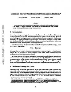
Single evaluation-based estimate. The first method, IBEA1 , consists in preserving the approach used in the deterministic case. A solution is evaluated only once and its fitness is estimated using this single evaluation (see fig. 1). Actually, most of the methods proceed like that since they are based on constant parameters and do not take uncertainties into account. The advantage of this method is its low computation cost, but the estimation error may be large since the evaluation used is not necessarily representative of the potential evaluation space. x2

f2

True evaluation One evaluation

Feasible solution

Decision space

Potential evaluation space

x1

Objective space

f1

Fig. 1. IBEA1 : a single evaluation is used to approximate the fitness of a solution

Average estimate. The second method, called IBEAavg , follows the idea commonly used in the single-criterion form and suggested in several multi-objective studies (such as, e.g., [1,5]). It consists in doing several evaluations of the same solution, and then in calculating the average value of these evaluations on each objective function. Next, the deterministic approach is applied using those average values (see fig. 2). This method also has the advantage of having a low computation cost if the evaluation of a solution is not too expensive (what is the case for our problem). However, losses of information may occur during the average estimate, like, e.g., the potential evaluations distribution in the research space.

Combinatorial Optimization of Stochastic Multi-objective Problems x2

f2

Potential evaluation space

Average evaluation

Feasible solution

463

True evaluation One evaluation

Decision space

x1

f1

Objective space

Fig. 2. IBEAavg : the average evaluation values are used to approximate the fitness of a solution

Probabilistic estimate. The last method consists in estimating the fitness of a solution in a probabilistic way. Here, contrary to some other approaches [10], we do not assume that there is a ‘true’ objective vector per solution which is blurred by noise, but we consider that a probability distribution is associated to each solution on the objective space (see fig. 3). In order to allow the comparison of potential values of solutions, this extension of IBEA, called IBEAstoch , consists in modifying the performance assessment procedure as proposed by Basseur and Zitzler in [2].

x2

f2

Potential evaluation space

p = 0.25 p = 0.25

True evaluation

Feasible solution

One evaluation p = 0.25 p = 0.25

Decision space

x1

Objective space

f1

Fig. 3. IBEAstoch: the fitness of a solution is estimated in a probabilistic way, a quality indicator being associated to each evaluation

A random variable F (x) is associated to each solution x ∈ X by the range of which is its corresponding potential evaluation space. The underlying probability distribution is usually unknown and may differ for other solutions. Thus, in practice, for a binary quality indicator I, the fitness of a solution x is computed using an estimation of expected I-values on a finite set of evaluations. Hence, for a population P = {x1 , x2 , . . . , xm } and a finite set of evaluation S(x), the fitness

464

A. Liefooghe et al.

of an individual x is defined as the estimated loss of quality if x is removed from the population, i.e.: ˆ Fitness(x) = E(I(F (P \ {x}), F (P )) ˆ = E(I(F (P \ {x}), F ({x}))  1 ˆ = |S(x)| z∈S(x) E(I(F (P \ {x}, {z}))) .

(8)

To compute the estimated expected I+ -value between a multiset A ∈ Ω and a reference objective vector z  , we consider all pairs (xj , zk ) where xj ∈ A and zk ∈ S(xj ) and sort them in the increasing order according to the indicator values I+ ({zk }, {z  }). Suppose the resulting order is (xj1 , zk1 ), (xj2 , zk2 ), . . . , (xjl , zkl ), the estimated expected I+ -value is then: ˆ + (F (A), {z ∗ })) = I+ ({zk1 }, {z ∗}) × Pˆ (F ({xj1 }) = {zk1 }) E(I + I+ ({zk2 }, {z ∗})× Pˆ (F ({xj2 }) = {zk2 }) | F({xj1 }) = {zk1 )}) + ... I+ ({zkl }, {z ∗})× Pˆ (F ({xjl }) = {zkl } | ∀1≤i5% ≡ > 5 % ≡ 0.009 − 0.013 + > 5 % ≡ 0.006 − 0.002 + 0.005 + 0.002 −

S metric IBEA1 IBEAavg p-value T p-value T 0.002 + 0.002 − 0.001 − 0.002 + 0.005 − 0.001 − 0.001 + 0.001 − 0.001 −

Table 2. Comparison of the quality assessment values obtained by IBEA1 , IBEAavg and IBEAstoch for exponentially distributed processing times using the Wilcoxon rank test

20 5 01 IBEAavg IBEAstoch 20 5 02 IBEAavg IBEAstoch 20 10 01 IBEAavg IBEAstoch

contribution metric IBEA1 IBEAavg p-value T p-value T >5% ≡ >5% ≡>5% ≡ >5% ≡ >5% ≡>5% ≡ 0.045 + 0.036 + > 5 % ≡

S metric IBEA1 IBEAavg p-value T p-value T 0.001 + > 5 % ≡ 0.033 − >5% ≡ 0.002 − 0.001 − 0.001 + > 5 % ≡ 0.005 −

468

A. Liefooghe et al.

Table 3. Comparison of the quality assessment values obtained by IBEA1 , IBEAavg and IBEAstoch for normally distributed processing times using the Wilcoxon rank test

20 5 01 IBEAavg IBEAstoch 20 5 02 IBEAavg IBEAstoch 20 10 01 IBEAavg IBEAstoch

contribution metric IBEA1 IBEAavg p-value T p-value T >5% ≡ >5% ≡>5% ≡ >5% ≡ >5% ≡>5% ≡ 0.004 + > 5 % ≡ 0.004 +

S metric IBEA1 IBEAavg p-value T p-value T 0.002 + 0.021 − 0.001 − 0.001 + 0.002 − 0.001 − 0.002 + 0.001 − 0.001 −

Table 4. Comparison of the quality assessment values obtained by IBEA1 , IBEAavg and IBEAstoch for log-normally distributed processing times using the Wilcoxon rank test

20 5 01 IBEAavg IBEAstoch 20 5 02 IBEAavg IBEAstoch 20 10 01 IBEAavg IBEAstoch

contribution metric IBEA1 IBEAavg p-value T p-value T >5% ≡ >5% ≡>5% ≡ >5% ≡ >5% ≡>5% ≡ >5% ≡ >5% ≡>5% ≡

S metric IBEA1 IBEAavg p-value T p-value T 0.032 − 0.001 − 0.001 − 0.001 + 0.001 + 0.001 − 0.001 + 0.001 + 0.020 −

Table 5. Comparison of the quality assessment values obtained by IBEA1 , IBEAavg and IBEAstoch for variously distributed processing times using the Wilcoxon rank test

20 5 01 IBEAavg IBEAstoch 20 5 02 IBEAavg IBEAstoch 20 10 01 IBEAavg IBEAstoch

contribution metric IBEA1 IBEAavg p-value T p-value T >5% ≡ >5% ≡>5% ≡ >5% ≡ >5% ≡>5% ≡ >5% ≡ >5% ≡>5% ≡

S metric IBEA1 IBEAavg p-value T p-value T 0.001 + 0.019 − 0.001 − 0.014 + > 5 % ≡ 0.010 − 0.001 + 0.003 + > 5 % ≡

The poor overall effectiveness of IBEAstoch can be partly explained by a low diversity among the Pareto set approximation obtained during the evaluation on the reference benchmark. Then, using an indicator that would increase the diversity in the decision space could give better results. Besides, the whole of the experimental results can be discussed as the evaluation protocol is not fully adapted to stochastic multi-objective problems.

Combinatorial Optimization of Stochastic Multi-objective Problems

5

469

Conclusion and Perspectives

In this paper, we investigated a bi-objective flow-shop scheduling problem with stochastic processing times as well as general combinatorial optimization algorithms applied to its resolution. First, we saw that, in real-world situations, none of the parameters related to this kind of problem is deprived of uncertainty. Thus, non-deterministic models are required to take this uncertainty into account. To this end, a proactive approach, where processing times are represented by random variables, have been taken and several general stochastic models have been proposed. Next, we introduced three different indicator-based methods for stochastic multi-objective problems that are able to handle any type of uncertainty. The first method, called IBEA1 , consists in preserving the deterministic approach by computing the fitness of a solution on a single evaluation. The second method, namely IBEAavg , is based on average objective values. At last, the IBEAstoch method consists in estimating the quality of a solution in a probabilistic way. The latter, already investigated in [2] on continuous problems, has never been applied neither to the combinatorial case nor to the stochastic models proposed here. All these algorithms and the fitness concept for multiobjective stochastic problems are now available within the ParadisEO-MOEO framework; new methods can thus easily be implemented in order to compare their effectiveness with those presented in this paper. To test these algorithms on our stochastic flow-shop problem, we initially had to build benchmark suites, first for the deterministic bi-objective case, then for the stochastic case. According to the experimental protocol we formulated, we concluded that IBEAavg was overall more efficient than IBEA1 and IBEAstoch . Even so, from a purely theoretical point of view, IBEAstoch seems to be more representative of the quality associated to a solution than the two other methods. In spite of that, the results it obtained are a little disappointing in comparison with the continuous case [2]; even if, in that last case, its effectiveness is especially significant for more than two objectives. This can be explained by the fact that the final solutions found by this algorithm are relatively close the ones from the others in the decision space, which generally implies, for our problem, that they are also close in the objective space. As a result, this method cannot contest the others in term of diversity. However, all these results should be moderated. No experimental protocol fully adapted to the combinatorial optimization of stochastic multi-objective problems exists up to now. The one we proposed, although simple and fast, is not really natural and is imperfectly adapted to this kind of problem. Moreover, considering the evaluation on the deterministic benchmark as the ‘true’ evaluation advantages a lot IBEAavg , especially for probability distributions whose central tendency is the mean. Different perspectives emerge from this work. First of all, other sources of uncertainty that processing times could be taken into account for the flow-shop problem. Furthermore, a reactive approach could be linked to our proactive approach in order to largely improve the effectiveness of all the algorithms. Additionally, as all the results obtained during our experiments reveal a weakness of convergence, hybridizing our evolutionary algorithms with local searches could

470

A. Liefooghe et al.

be beneficial, especially to accelerate the exploration near potentially interesting solutions. Moreover, even if most of quality indicators to be used with IBEA take diversity into account, they only deal with diversity on the objective space, and not on the decision space. Then, to fill the low-level of diversity of IBEAstoch , it could be interesting to create an indicator that would allow the decision maker to obtain diversified solutions in the decision space and that would not be completely focused on the Pareto dominance relation. Also, perhaps IBEAstoch is simply to fine-grained compared to IBEAavg , and so presents a landscape with a complex structure whereas IBEAavg provides a reasonable guidance and uses stochasticity to pass over such a structure. Studying the lanscape more precisely could then be helpful. Besides, the population size as well as the number of evaluations per solution are two parameters that influence a lot the effectiveness of all the algorithms. Studying more finely the way of determining them and analyzing how to make them evolve in a more efficient way during the optimization process could be profitable. Lastly, working out an experimental protocol adapted to the combinatorial optimization of stochastic multi-objective problems proves to be essential to evaluate the results in a more rigorous way. As well, this study could be extended in order to consider problems with more than two ojectives.

References 1. Babbar M., Lakshmikantha A., Goldberg D. E.: A Modified NSGA-II to Solve Noisy Multiobjective Problems. In Foster J. et al. (eds.): Genetic and Evolutionary Computation Conference (GECCO’2003). Lecture Notes in Computer Science 2723, Springer, Chicago, Illinois, USA (2003) 21–27 2. Basseur M., Zitzler E.: Handling Uncertainty in Indicator-Based Multiobjective Optimization. International Journal of Computational Intelligence Research 2(3) (2006) 255–272 3. Cunningham A. A., Dutta S. K.: Scheduling jobs with exponentially distributed processing times on two machines of a flow shop. Naval Research Logistics Quarterly 16 (1973) 69–81 4. Dauz`ere-P´er`es S., Castagliola P., Lahlou C.: Niveau de service en ordonnancement stochastique. In Billaut J.-C. et al. (eds.): Flexibilit´e et robustesse en ordonnancement. Herm`es, Paris (2004) 97–113 5. Deb K., Gupta H.: Searching for Robust Pareto-Optimal Solutions in MultiObjective Optimization. In Coello Coello C. A. et al. (eds.): Evolutionary MultiCriterion Optimization, Third International Conference (EMO 2005). Lecture Notes in Computer Science 3410, Springer, Guanajuato, Mexico (2005) 150–164 6. Dudek R. A., Panwalkar S. S., Smith M. L.: The Lessons of Flowshop Scheduling Research. Operations Research 40(1), INFORMS, Maryland, USA (1992) 7–13 7. Graham R. L., Lawler E. L., Lenstra J. K., Rinnooy Kan A. H. G.: Optimization and Approximation in Deterministic Sequencing and Scheduling: A Survey. Annals of Discrete Mathematics 5 (1979) 287–326 8. Hughes E. J.: Evolutionary Multi-Objective Ranking with Uncertainty and Noise. In Zitzler E. et al. (eds.): Evolutionary Multi-Criterion Optimization, First International Conference (EMO 2001). Lecture Notes in Computer Science 1993, Springer, London, UK (2001) 329–343

Combinatorial Optimization of Stochastic Multi-objective Problems

471

9. Ishibuchi H., Murata T.: A Multi-Objective Genetic Local Search Algorithm and Its Application to Flowshop Scheduling. IEEE Transactions on Systems, Man and Cybernetics 28 (1998) 392–403 10. Jin, Y., Branke, J.: Evolutionary Optimization in Uncertain Environments - A Survey. IEEE Transactions on Evolutionary Computation 9 (2005) 303–317 11. Keijzer M., Merelo J. J., Romero G., Schoenauer M.: Evolving Objects: A General Purpose Evolutionary Computation Library. Proc. of the 5th International Conference on Artificial Evolution (EA’01), Le Creusot, France (2001) 231–244 12. Kouvelis P., Daniels R. L., Vairaktarakis G.: Robust scheduling of a two-machine flow shop with uncertain processing times. IIE Transactions 32(5) (2000) 421–432 13. Ku P. S., Niu S. C.: On Johnson’s Two-Machine Flow Shop with Random Processing Times. Operations Research 34 (1986) 130–136 14. Landa Silva J. D., Burke E. K., Petrovic S.: An Introduction to Multiobjective Metaheuristics for Scheduling and Timetabling. In Gandibleux X. et al. (eds.): Metaheuristics for Multiobjective Optimisation. Lecture Notes in Economics and Mathematical Systems 535, Springer, Berlin (2004) 91–129 15. Meunier H., Talbi E.-G., Reininger P.: A multiobjective genetic algorithm for radio network optimization. In Proc. of the 2000 Congress on Evolutionary Computation (CEC’00). IEEE Press (2000) 317–324 16. T’kindt V., Billaut J.-C.: Multicriteria Scheduling - Theory, Models and Algorithms. Springer, Berlin, 2002. 17. Taillard E. D.: Benchmarks for Basic Scheduling Problems. European Journal of Operational Research 64 (1993) 278–285 18. Teich J.: Pareto-Front Exploration with Uncertain Objectives. In Zitzler E. et al. (eds.): Evolutionary Multi-Criterion Optimization, First International Conference (EMO 2001). Lecture Notes in Computer Science 1993, Springer, London, UK (2001) 314–328 19. Zitzler E., Thiele L.: Multiobjective Evolutionary Algorithms: A Comparative Case Study and the Strength Pareto Approach. IEEE Transactions on Evolutionary Computation 3(4) (1999) 257–271 20. Zitzler E., Thiele L., Laumanns M., Fonseca C. M., Grunert da Fonseca V.: Performance Assessment of Multiobjective Optimizers: An Analysis and Review. IEEE Transactions on Evolutionary Computation 7(2) (2003) 117–132 21. Zitzler E., K¨ unzli S.: Indicator-Based Selection in Multiobjective Search. In Parallel Problem Solving from Nature (PPSN VIII). Lecture Notes in Computer Science 3242, Springer, Birmingham, UK (2004) 832–842