The (hypothetical) noise-free image that can be ob- served from this camera is ... PDF with mean µ and covariance Σ, and let g(.; hk) be the outlier distribution ...
Combined Depth and Outlier Estimation in Multi-View Stereo Christoph Strecha, Rik Fransens and Luc Van Gool K.U.Leuven-ESAT-Psi Kasteelpark 1, 3001 Leuven, Belgium
Abstract In this paper, we present a generative model based approach to solve the multi-view stereo problem. The input images are considered to be generated by either one of two processes: (i) an inlier process, which generates the pixels which are visible from the reference camera and which obey the constant brightness assumption, and (ii) an outlier process which generates all other pixels. Depth and visibility are jointly modelled as a hidden Markov Random Field, and the spatial correlations of both are explicitly accounted for. Inference is made tractable by an EM-algorithm, which alternates between estimation of visibility and depth, and optimisation of model parameters. We describe and compare two implementations of the E-step of the algorithm, which correspond to the Mean Field and Bethe approximations of the free energy. The approach is validated by experiments on challenging real-world scenes, of which two are contaminated by independently moving objects. Figure 1. Semper statue scene: combined depth and outlier estimation. Left: input images, the middle is choosen as the reference view. Right: depth and outlier estimates.
1. Introduction Computing depth from stereo images remains a difficult problem to solve because of several reasons. First of all, the stereo problem is ill-posed and has inherent ambiguities. Secondly, image noise, as well as the complexity of 3D scenes, make it difficult to develop algorithms which produce good results over a large variety of input images. Finally, occlusions further complicate or even render impossible the extraction of depth. To deal with the ill-posedness of the stereo problem, most algorithms incorporate some form of regularisation. In global approaches, such as Markov Random Field (MRF) formulations, regularisation is implemented by defining a suitable Gibbs prior which favours spatially smooth field configurations. In local methods, such as Partial Differential Equation (PDE) formulations, regularisation is performed by introducing a regularisation term in the matching energy. Often, however, the need for regularisation leads to an excess of parameters, which have to be carefully tuned to
obtain the desired performance. The formulation of a multiview stereo algorithm in a Bayesian framework alleviates this problem to some extent. For example, deviations from model assumptions are typically captured by a noise term, and the optimal noise level can be estimated by maximumlikelihood (ML) estimation from the data itself. The occlusion problem is often viewed from a geometric perspective only. However, it can be more generally described as an outlier problem. Outliers can be devided into three types, examples of each of which are present in fig.(1): (i) geometrical occlusions, which have their origin in the 3D-structure of the scene, (ii) objects like pedestrians or cars, whose relative location in the scene changes while the images are captured, and (iii) violations of the constant 1
brightness assumption, like specular reflections or discretisation errors. In what follows, we will jointly refer to outlier pixels as ‘invisible’ pixels. Previous work on dealing with outliers in multi-view stereo can be divided into three categories. The first category consists of algorithms which perform explicit geometrical computations, by tracing the lines of sight from the current depth solution to the input images and verifying if there exist crossings with this solution. Examples are methods using MRF’s [12], level-sets [3, 11, 17] or voxel coloring [14]. In the second category we find algorithms which rely on consistency checks to detect outliers. Depth is computed w.r.t. each input image, and outliers are identified by inconsistencies in the extracted depth maps [6, 8, 10, 7]. The third category consists of algorithms which use photometric cues. For example, robust kernel methods [9] use a matching kernel which diminishes the influence of outlier pixels. Often, pixel matches which fall below a certain threshold [22, 13] are ignored all together. Such a threshold disappears in generative model based formulations as proposed in our previous work [19]. An extension of this also incorporates geometric cues [7]. Wheras the first category focusses on geometric occlusions, the second and third category can in principle handle all types of outliers. Most of the above algorithms separate the computation of depth and visibility. However, this separation introduces a notorious ‘chicken and egg’ problem: knowledge of depth is needed to compute outliers, and outliers must be identified to compute a reliable depth. Many algorithms therefore estimate both in turn, which is a reasonable approach if the amount of occlusions or outliers is small. For example, in Kang et al. [12], the starting point is the estimation of depth under the assumption that everything is visible. Next, visibilities are estimated and depth is re-computed, keeping the best-matching depths from the previous solution fixed. This procedure is iterated and progressively more points are added to the solution. By contrast, we propose to jointly model depth and visibility and try to identify the most likely joint configuration, given the input images. We define a generative model, in which the input images are assumed to be generated by either an inlier process or an outlier process [19, 4]. The inlier process is responsible for the generation of pixels for which stereo correspondence can be established, i.e. which are visible from the reference camera and which obey the constant brightness assumption. The outlier process, on the other hand, is responsible for the generation of pixels for which no correspondence can be established. Depth and visibility are jointly modelled as a hidden Markov Random Field, and the spatial correlations of both are explicitly accounted for by defining a suitable Gibbs prior distribution. The ML-estimates of the statistics of the inlier and outlier processes are obtained by an Expectation-Maximisation
(EM) algorithm [2]. This algorithm keeps track of which points of the scene are visible in which images, and accounts for all likely visibility configurations. Therefore, it can deal with scenes which are contaminated by independently moving objects, such as pedestrians or cars whose relative location in the scene changes while the images are captured. This is a rare feature, which often proves useful, especially when dealing with outdoor-scenes. We experiment with two implementations of the E-step of the algorithm, corresponding to the Mean Field and Bethe approximations of the free energy. The impact of this choice is validated on groundtruth data.
2. Probabilistic Model 2.1. Problem Statement We are given K images yk , k ∈ [1, ..., K], which are taken with a set of cameras of which we know the internal and external calibrations. Each image consists of a set of pixel values over a rectangular lattice and will be denoted as yk = {yik }, where i indexes the nodes of the lattice. The objective is to compute the depth of the scene in such a way that the information of all images contributes to the final solution. Depth is computed w.r.t. a particular camera, which could be one of the cameras from which the input images are taken, but which could equally well be a virtual camera representing a view point not available in the set of input images. The (hypothetical) noise-free image that can be observed from this camera is referred to as the ideal image and will be denoted as y∗ = {yi∗ }. The multi-view stereo problem now consists of computing those depth values which map the pixels yi∗ of the ideal image onto similarly coloured pixels yik� in all input images 1 .
2.2. Generative Imaging Model In this paper, we take a generative model based approach to solve the multi-view stereo problem. The input images are considered to be generated by either one of two processes: (i) an inlier process which generates the pixels yik which are visible from the camera related to y∗ and which obey the constant brightness assumption, and (ii) an outlier process which generates all other pixels. The inlier process is modelled as: (1) yik� = yi∗ + � , where � is image noise which is assumed to be normally distributed with zero mean and covariance Σ. The outlier process is modelled as a random generator, sampling from 1 Given the camera calibrations, it is easy to compute the locations corresponding to yi∗ in the other images, see for example [19].
K unknown distributions characterised by probability density functions (PDFs) g k . These PDFs are modelled as histograms and are parametrised by the histogram entries hk . Associated with the ideal image y∗ is a hidden Markov Random Field (MRF) x = {xi }, where i again indexes the nodes of the lattice. This random field represents the unobservable state of each node. Traditionally, the state of a node corresponds to its depth-value. Suppose depth is discretised into R levels, then each element xi is defined to be a binary random R-vector, i.e. xi = [x1i . . . xri . . . xR i ], of which exactly one element is 1 and all others are 0. The position of the 1 indicates the depth-value of the pixel. Furthermore, a smoothness constraint is imposed by defining a Gibbs prior distribution on x which favours spatially smooth random field configurations. In this paper, we augment this representation and consider the state of a pixel to be a combination of its depth and its visibility configuration. The visibility configuration of the ith pixel specifies in which of the K input images it is visible. In principle, the total number of visibility configurations is 2K . However, certain configurations, in which the pixel is visible in less than a predescribed number of images, are not very likely and will not be considered. Let S denote the number of visibility configurations under consideration and let s be an index over these configurations. Then the sth configuration of the ith pixel can be represented by a binary K-vector vis = [vis1 . . . visk . . . visK ], in which each element signals whether or not the pixel is visible in the respective image. The state of a pixel is a combination of its discrete depth and its visibility configuration, and the number of possible states is M = RS. The state of the ith pixel is represented M by the binary M -vector xi = [x1i . . . xm i . . . xi ], of which exactly one element is 1. Sometimes, we will find it convenient to index these elements with the double index rs, in which r refers to the depth level and s refers to the visibility configuration. The conversion between single and double indexing is given by m = (r − 1)S + s. A smoothness constraint is imposed on the random field x by defining a suitable Gibbs prior distribution. This distribution, which will be specified in the next section (2.3), favours random field configurations in which neighbouring pixels have similar depths and similar visibility configurations. We are now in the position to describe the probabilistic model in more detail. Let f (.; µ, Σ) denote a normal PDF with mean µ and covariance Σ, and let g(.; hk ) be the outlier distribution associated with the k th image. Furthermore, let xrs i be the element of the state vector xi which is 1 and let yik� be the pixel in the k th image onto which yi∗ is mapped. Then the probability of observing yik� , conditioned on the unknowns θ = {y∗ , Σ, hk } and the state of the MRF x, is given by: � f (yik� ; yi∗ , Σ) if visk = 1 k (2) p(yi� |θ, x) = g(yik� ; hk ) if visk = 0
2.3. Markov Random Field Gibbs Prior In the previous section we introduced the MRF x which represents the unobservable state of each pixel in the ideal image y∗ , where the state of a pixel is a combination of its discrete depth and its visibility configuration. According to the Hammersley-Clifford theorem, the prior distribution p(x) is a Gibbs distribution which factorises over the cliques of the graph. Let Ni represent a 4-neighbourhood of the ith node, i.e. Ni is the set of indices of the nodes directly above, below, left and right of the ith node. The Gibbs prior is given by: 1 � � ψ(xi , xj ) , (3) p(x) = Z i j∈Ni
where Z is a normalisation constant (the ’partition function’) and ψ is an interaction potential. The latter is a positive valued function defined over the cliques of the graph, and embodies the prior beliefs about the smoothness of the random field. In our case, the interaction potential should consider both the depths and the visibility configurations of neighbouring nodes. Suppose node i is in the rsth state and has discrete depth dir and visibility configuration vis . Furthermore, suppose node j is in the pq th state and has discrete depth djp and visibility configuration vjq . The distance Dij (r, p) between two depth labels r, p of neighbouring nodes i and j is defined by the L1 norm | r − p | /R. Since the discrete depth values d r are sampled uniformly on an inverse depth scale, this choice leads to a smooth disparity. The distance Dij (s, q) between two visibility configurations s, q is defined as the number of dissimilar entries of vis and vjq . Furthermore we introduce a constant C with accounts for non smooth cliques interactions. The interaction potential has the following form: pq ψ(xrs i , xj ) = e
−
Dij (r,p) σd
e−
Dij (s,q) σv
+C ,
(4)
where σd and σv are proportional to the standard deviations of the Laplace distributions. Note that this interaction can be derived from a generative model (similar to (2)) of depth and visibility under a Laplacian noise distribution and with outlier probability C [5]. It has also strong similarities to [9].
3. Maximum Likelihood Estimation Let θ = {y∗ , Σ, hk } denote all unknowns, and let y = {y } denote all input data. The maximum-likelihood (ML) estimate of the unknowns is given by: � � θ�ML = arg max log p(y | θ) θ � � � p(y | x, θ) p(x) , (5) = arg max log k
θ
x
where the assumption was made that the random field x is independent from θ. Conditioned on the state of the hidden variables x, the data-likelihood factorises as a product over all individual pixel likelihoods: �� p(y | x, θ) ≈ p(yik� | xi , θ) i
=
k
��� i
k
m
xi p(yik� | xm . i , θ)
(6)
m
In the product over m, only the factor for which xm i = 1 survives. Notice that the data-likelihood factorisation is only approximately correct, because in general pixels yi∗ in the ideal image will not map onto integral positions in the input images yk . Depending on the relative positions and orientations of the cameras, this will lead to overusage or underusage of the pixels yik . Each binary index xm i corresponds to a particular discrete depth value dir and visibility configuration vis = [vis1 . . . visk . . . visK ]. Based on these visibility values, the pixel-likelihood in the right hand side of eq. (6) can be further expanded as: � �visk � �1−visk k ∗ k k g(y p(yik� | xm , θ) = f (y ; y , Σ) ; h ) . � � i i i i
(7)
We have now specified all terms of the data-likelihood p(y | θ). However, the sum x in the right hand side of eq. (5) ranges over all possible configurations of the random field x. Even for modest sized images, the total number of configurations of x is huge, hence direct optimisation of the log-likelihood is infeasible. The Expectation-Maximisation (EM) algorithm offers a solution to this problem, essentially by replacing the logarithm of a large sum into the expectation of the log-likelihood.
3.1. EM Algorithm It was shown by Neal and Hinton [15] that the EM algorithm can be viewed in terms of ’free energy’ minimisation, where the free energy is defined as follows: p) . F (˜ p, θ) = −Ep˜[log p(y, x | θ))] − H(˜
(8)
Here, p˜ is some distribution over the hidden variables x, p) is the Ep˜[ ] denotes the expectancy under p˜, and H(˜ entropy of p˜. Starting from an initial parameter guess θˆ(0) , the EM algorithm generates a sequence of parameter estimates θˆ(t) and distribution estimates p˜(t) by alternating the following two steps: p, θˆ(t) ). E-step Set p˜(t) to that p˜ which minimises F (˜ (t+1) ˆ M-step Set θ to that θ which minimises F (˜ p(t) , θ). Moreover, the authors prove that in the E-step, the
minimiser of F (˜ p, θ) is given by the true posterior distri(t) ˆ bution p(x | y, θ ). In order to compute this posterior in a tractable manner, it is often approximated by a simpler, factorisable distribution h(x). The task then is to find h(x), which is as close as possible to the true posterior, where the distance between both distributions is measured by the Kullback-Leibler divergence. The minimum of the Kullback-Leibler divergence is directly related to the minimum of the free energy [15, 21]. In the mean field approximation, p(x | y, θˆ(t) ) is approximated by a distribution h(x) which fully factorises over the nodes of the lattice: � hi (xi ) , (9) h(x) = i
where hi is a distribution over the M possible states of the ith node. It is specified by an M -vector of one-node beliefs M m [b1i . . . bm i . . . bi ], in which bi is the probability that node i is in state m. Let ψmn denote the value of the interaction potential ψ(xi , xj ) when nodes i and j are in the mth and nth state, respectively. Then the mean field free energy FMF is, upto a constant, given by: ��� k m FMF = − bm i log p(yi� | xi , θ) i
−
i
+
k
m
��� �� i
n bm i bj log ψmn
j∈Ni m,n m bm i log bi .
(10)
m
The first two terms of FMF correspond to the expected value of the log-likelihood (the so-called Q-function), and the last term is the negative entropy of x under h(x). In the E-step, the free energy is minimised w.r.t. the distribution h(x), where we use the current estimates θˆ(t) for θ. This is achieved by setting the derivatives ∂FMF /∂bm i to zero, and leads to the update equations: �
�� � k n ˆ(t) ) exp . ← p(y | x , θ b log ψ bm � i mn i i j j∈Ni n
k
(11) After these updates, the beliefs are renormalised as to fulfil the normalisation condition m bm i = 1. These equations are solved by iterative re-substitution, which converges fast. At the end of the E-step, for each node i we can compute the depth Di and visibility Vik w.r.t. the k th image in two ways. First of all, we could only consider the state with maximal belief, say xrs i , and use the depth and visibility configuration of this state: Di = dir and Vik = visk . Alternatively, we could compute the expected depth and visibility by considering all states: � � r sk brs Vik = brs (12) Di = i di , i vi . rs
rs
The last method has the advantage of generating smoother and non-discrete depth estimates. However, if multimodalities exist in the posterior beliefs bm i , the estimate might be wrong. In the M-Step, the free energy is optimised w.r.t. the parameters θ. This is achieved by setting each parameter θ to the appropriate root of the derivative equation ∂FMF /∂θ = 0. The update equations for the ideal image and noise covariance are: k k k Vi yi� yi∗ = k k Vi k k ∗ k ∗ T i k Vi (yi� − yi )(yi� − yi ) k Σ = , (13) i k Vi where Vik are the expected visibilities computed according to eq.(12). The histogram entries of the outlier distributions g(.; hk ) are updated as follows. Suppose the colour space is discretised into B bins, i.e. hk = {hkb }, b ∈ [1. . .B]. Maximisation of FMF w.r.t. the histogram entries hkb , subject to the constraint that all entries should sum to the inverse bin volume, results in: � (1 − Vik ) δb (yik� ) , (14) hkb ∝ i
where δb (yik� ) is an indicator function which evaluates to 1 if the pixel value falls in the bth bin and evaluates to 0 otherwise. Put differently, hk is a histogram of the k th input image, where the data yik� are weighted by their probability of being not visible. The E and M-step are alternated until the relative change of the parameters θ falls below a prespecified threshold. Alternatively, in the Bethe approximation p(x | y, θˆ(t) ) is approximated by a distribution h(x) which factorises as follows [21]: ij hij (xi , xj ) . (15) h(x) = qi −1 i hi (xi ) Here, qi is the size of the neighbourhood (4 in our case) and hij (xi , xj ) is a joint distribution over the states of neighbouring nodes. It is specified by the M ×M -matrix of twonode beliefs bmn ij , which specify the probability that node i is in state m and node j is in state n. The Bethe free energy is a function of the one-node and two-node beliefs: ��� k m bm FB = − i log p(yi� | xi , θ) i
−
i
+
k
m
��� �
j∈Ni m,n
(qi − 1)
�
i
+
��� i
bmn ij log ψmn
j∈Ni m,n
m bm i log bi
m mn bmn ij log bij .
(16)
Again, the first two terms of FB correspond to the expected value of the log-likelihood, and the last two terms specify the negative entropy of h(x). The Bethe free energy is exact for graphs without loops [21]. For graphs with loops, like in our case, it is an approximation of the true free energy. It was recently shown that the popular belief propagation algorithm, introduced by Pearl [16], minimises the Bethe free energy w.r.t. respect to bi and bij [21]. The EMalgorithm proceeds by iterating the following steps. In the E-Step, the Bethe free energy is minimised w.r.t. bi and bij by belief propagation. In the M-Step, the parameters are updated according to eqs. (13) and (14). The updates of the parameters are the same for both free energy approximations, because they only appear in the terms of FMF and FB which correspond to the expected value of the loglikelihood.
4. Experimental Validation In our experiments we do not consider all possible visibility configuration of a pixel, since some of them are very unlikely. Consider the case of three images yk in which there are 8 possible visibility configurations vis for every pixel yi∗ in the ideal image. These configurations are shown in table (1). Depending on the application we can distiny1 y2 y3
vi1 1 1 1
vi2 1 1 0
vi3 1 0 1
vi4 1 0 0
vi5 0 1 1
vi6 0 1 0
vi7 0 0 1
vi8 0 0 0
Table 1. Possible visibility configurations for three images. guish between two scenarios. The first scenario is the most general one. The reference camera is one of the input cameras or a virtual camera, and there might be independently moving objects in the scene. This implies that one cannot assume that all pixels yi∗ from the ideal image are simultaneously visible in one of the input images yk . To be able to assign a meaningful depth and colour to an ideal image pixel yi∗ , it must be visible in at least two images. Configurations in which a pixel is visible in only one image are in principle possible, but are in reality not very likely to occur. Therefore, we only consider the visibility configurations given by s = {1, 2, 3, 5}. By using these configurations, it is possible to remove independently moving objects from the scene and still compute a depth value at these outlier pixels. In the second scenario, the reference camera is one of the input cameras, say y1 , and if there are independently moving objects in the scene they are not visible from the reference camera. In this particular case, all pixels yi∗ are by
Bethe Mean Field error σd = 300 σd = 400 σd = 300 σd = 400 1.0/0.5 3.83/8.43 3.71/7.68 13.2/22.1 10.1/18.9 Table 2. Results for Bethe and mean field approximation on Cones ground truth data.
The results for two view stereo on the whole Middlebury set, all processed with σd = 300, σv = 30, Cs = 10−10 , Cd = 10−4 , are shown in table (3). We report the percentage of pixels with a disparity error larger than 1 and larger than 0.5, evaluated at all pixels for which correspondence can be established. Figure 2. Comparison of Bethe (top) and mean field (bottom) approximation: depth (left) and detected occlusions (right).
error 1.0/0.5
Tsukuba Venus Teddy Cones 2.57/7.89 1.72/4.59 6.86/14.8 4.64/10.2
Table 3. Middlebury stereo evaluation. definition visible in y1 (the geometrical transformation between y∗ and y1 is the identity transformation), which puts stronger constraints on the possible solutions. The possible visibility configurations vis are given by s = {1, 2, 3, 4}. In this case we are now able to explicitly identify the regions for which no depth estimation is possible (s = 4). In order to model discontinuities of the MRF we use two interaction matrices, which differ by the constant C in eq. (4). The first (C = Cd ) is used for all cliques for which the endpoints fall into a different mean shift colour segment [1], and the second (C = Cs ) for the remaining cliques.
4.1. Ground truth Evaluation In the first experiment we compare the quality of the mean field with the Bethe approximations on the ‘cones sequence’ of the Middlebury Stereo evaluation set [18]. Three images have been used with visibility configurations s = 1, 2, 3 and parameters σd = 400, σv = 30, Cs = 10−10 , Cd = 10−4 . The extracted depth and visibility for the images which are used in the Middlebury set are shown in fig. (2). Table (2) compares both approximation by the percentage of pixels with a disparity error large than 1 and larger than 0.5, evaluated for all visible pixels (equivalent to [18]). The best result was obtained by the Bethe approximation, which is in agreement with the results of Weiss on other inference problems [20]. The occlusions are detected well as long as the occluded parts contains textural information. For homogeneous occluded regions a match at a wrong depth is estimated as being more likely.
4.2. Outdoor Scene Reconstructions We tested our algorithm on several challenging outdoor scenes, characterised by multiple depth occlusions, independently moving objects and complicated scene geometry. The first example shows a scene which is contaminated by pedestrians. The three input images are shown in the top row of fig. (3). The camera position of the ideal image was chosen to be the left of these images. Notice that all images are contaminated with independently moving objects. Also the reference image contains pixels (e.g. woman in white) which have no support in any other image. Still, the results in fig. (4) show that our algorithm could assign a meaningful colour (left) and depth (right) to those outlier pixels. The bottom row in fig. (3) shows the visibility estimates. The Bethe approximation of the free energy was used, and four visibility configurations v s , s = 1, 2, 3, 5 were considered. The depth estimation at the bottom of the ideal image y∗ is rather poor. The reason for this is the lack of texture and the fact that the epipole lies within all target images. However, the ideal image looks visually convincing and the estimated depth, visibility and ideal image constitute a solution which makes the input images very likely. In the next experiment we used three images of the ‘cityhall scene’ [19]. These images are shown in the top row of fig. (5). Because this scene does not contain independently moving objects, we only consider the three visibility configurations v s , s = 1, 2, 3 in table (1). In the bottom row the extracted depth and visibilities are shown. We used the Bethe approximation with parameters σd = 300, σv =
Figure 3. Top: the three input images. The camera position of the virtual image y∗ was chosen to be the left of these images. Bottom: visibility estimates related to y∗ .
30, Cs = 10−10 , Cd = 10−4 . For the experiment in fig. (1) the same visibility configurations were considered. Both experiments show excellent depth and visibility estimates. The datasets (images, calibration and calibration points) are available at www.esat.kuleuven.be/∼cstrecha/testimages.
5. Discussion and Conclusions We presented a new approach to multi-view stereo which can deal with scenes that are contaminated by accidental objects. A novel view is computed, which is most likely given the input images. To compute this view, all possible configurations of depth and visibilities are taken into account. This results in the elimination of accidental objects which cannot be explained by the majority of input images. Most existing multi-view stereo algorithms compute depth w.r.t. the reference image itself, and therefore lack this ability. Novel view synthesis in conjunction with depth estimation has been formulated in [19] and further extended in [7]. Both methods use a PDE solution scheme. Being local methods, memory and CPU demands are relatively low, hence depth can be computed for large images. However, they also rely on a good initialisation in order to converge. Global formulations like MRF, on the other hand, have been shown to convergence well even without initial depth estimate. They could therefore be used as an initialisation for a local optimisation scheme on high resolution images.
Figure 4. Ideal image y∗ and depth estimate, computed from the three input images shown in fig. (3). Notice that the woman has disappeared from y∗ and that a depth and colour value is assigned to these pixels by matches in the other views.
In the E-step of the EM algorithm, we experimented with two approximations of the free energy: the mean field and Bethe approximation. Minimising the latter energy can be achieved by belief propagation. We numerically evaluated the quality of both approximations on ground truth data. This showed that for the stereo problem, the Bethe approximation has clear advantages over the mean field approximations. The results also show that our method scores well on the Middlebury stereo evaluation. Currently, we are at the fourth position when performance is measured at the highest precision (0.5 pixels disparity error) for all visible pixels. The presented approach to detect outliers is purely based on photometric cues. Therefore, it can cope with independently moving objects, as well as geometric occlusions. For example, photometric cues are necessary to deal with scenes like the one shown in fig. (3). However, when the scene contains large untextured regions, photometric cues could fail to detect an occlusion. It remains possible that the occlusion can be explained by assigning a wrong depth, if this provides a consistent match in all images. An example of this can be observed at the left side of the front-right cone in fig. (2). Combining photometric and geometric cues is expected to further increase the robustness of outlier detection. This combination will be considered in future work. Acknowledgement: The authors gratefully acknowledge support by KUL-GOA Marvel, FWO and Pascal.
Figure 5. Cityhall scene. Top: the three input images, the camera position of ideal image y∗ was chosen to be the left image. Bottom: estimated depth and visibility.
References [1] D. Comaniciu and P. Meer. Mean shift: A robust approach toward feature space analysis. PAMI, 24(5):603–619, 2002. [2] A. Dempster, N. Laird, and Rubin.D.B. Maximum likelihood from incomplete data via the EM algorithm. J. R. Statist. Soc. B, 39:1–38, 1977. [3] O. D. Faugeras and R. Keriven. Complete dense stereovision using level set methods. ECCV, 1:379–393, 1998. [4] R. Fransens, C. Strecha, and L. Van Gool. A mean field EM-algorithm for coherent occlusion handling in mapestimation problems. CVPR, page (this proccedings), 2006. [5] R. Fransens, C. Strecha, and L. Van Gool. Robust estimation in the presence of spatially coherent outliers. to appear, 2006. [6] P. Fua. A parallel stereo algorithm that produces dense depth maps and preserves image features. Machine Vision and Applications, 6(1):35–49, 1993. [7] P. Gargallo and P. Sturm. Bayesian 3d modeling from images using multiple depth maps. CVPR, 2:885–891, 2005. [8] D. Geiger, B. Ladendorf, and A. Yuille. Occlusions and binocular stereo. IJCV, 14(3):211–226, 1995. [9] S. Jian, Z. Nan-Ning, and S. Heung-Yeung. Stereo matching using belief propagation. PAMI, 25(7):787–800, 2003. [10] S. Jian, L. Yin, and K. Sing Bing. Symmetric stereo matching for occlusion handling. CVPR, 2:399–406, 2005. [11] H. Jin, A. Yezzi, and S. Soatto. Variational multiframe stereo in the presence of specular reflections. 3DPVT, pages 626– 630, 2002. [12] S. Kang, R. Szeliski, and J. Chai. Handling occlusions in dense multi-view stereo. CVPR, 1:103–110, 2001.
[13] V. Kolmogorov and R. Zabih. Multi-camera scene reconstruction via graph cuts. ECCV, 3(3):82–96, 2002. [14] K. Kutulakos and S. Seitz. A theory of shape by space carving. IJCV, 38(3):197–216, 2000. [15] R. M. Neal and G. E. Hinton. A view of the EM algorithm that justifies incremental, sparse, and other variants, pages 355–368. MIT Press, Cambridge, MA, USA, 1999. [16] J. Pearl. Probabilistic Reasoning in Intelligent Systems: Networks of Plausible Inference. Morgan Kaufmann Publishers Inc., San Francisco, CA, USA, 1988. [17] J.-P. Pons, R. Keriven, and O. D. Faugeras. Modelling dynamic scenes by registering multi-view image sequences. CVPR, 2:822–827, 2005. [18] D. Scharstein and R. Szeliski. A taxonomy and evaluation of dense two-frame stereo correspondence algorithms. IJCV, 47(1/2/3):7–42, 2002. [19] C. Strecha, R. Fransens, and L. Van Gool. Wide-baseline stereo from multiple views: a probabilistic account. CVPR, 1:552–559, 2004. [20] Y. Weiss. Comparing the mean field method and belief propagation for approximate inference in MRFs. Saad D. and Opper M. MIT Press, 2001. [21] J. S. Yedidia, W. T. Freeman, and Y. Weiss. Understanding belief propagation and its generalizations, pages 239–269. Morgan Kaufmann Publishers Inc., 2003. [22] C. Zitnick and T. Kanade. A cooperative algorithm for stereo matching and occlusion detection. PAMI, 22(7):675 – 684, 2000.