Combining block-based and online methods in learning ensembles ...

NOTICE: this is the authors version of a work that was accepted for publication in Information Sciences. Changes resulting from the publishing process, such as peer review, editing, corrections, structural formatting, and other quality control mechanisms may not be reflected in this document. Changes may have been made to this work since it was submitted for publication. DOI: http://dx.doi.org/10.1016/j.ins.2013.12.011

Combining block-based and online methods in learning ensembles from concept drifting data streams Dariusz Brzezinski∗, Jerzy Stefanowski Institute of Computing Science, Poznan University of Technology, ul. Piotrowo 2, 60–965 Poznan, Poland

Abstract Most stream classifiers are designed to process data incrementally, run in resource-aware environments, and react to concept drifts, i.e., unforeseen changes of the stream’s underlying data distribution. Ensemble classifiers have become an established research line in this field, mainly due to their modularity which offers a natural way of adapting to changes. However, in environments where class labels are available after each example, ensembles which process instances in blocks do not react to sudden changes sufficiently quickly. On the other hand, ensembles which process streams incrementally, do not take advantage of periodical adaptation mechanisms known from block-based ensembles, which offer accurate reactions to gradual and incremental changes. In this paper, we analyze if and how the characteristics of block and incremental processing can be combined to produce new types of ensemble classifiers. We consider and experimentally evaluate three general strategies for transforming a block ensemble into an incremental learner: online component evaluation, the introduction of an incremental learner, and the use of a drift detector. Based on the results of this analysis, we put forward a new incremental ensemble classifier, called Online Accuracy Updated Ensemble, which weights component classifiers based on their error in constant time and memory. The proposed algorithm was experimentally compared with four state-of-the-art online ensembles and provided best average classification accuracy on real and synthetic datasets simulating different drift scenarios. Keywords: concept drift, data streams, online classifier, ensembles

1. Introduction For the last decades, several machine learning and data mining algorithms have been proposed to discover knowledge from data [26, 18, 17]. However, such algorithms are usually applied to static, complete datasets, while in many new applications one faces the problem of processing massive data volumes in the form of transient data streams. Example applications involving processing data generated at very high rates include sensor networks, telecommunication, GPS systems, network traffic management, and customer click logs. The processing of streaming data implies new requirements concerning limited amount of memory, small processing time, and one scan of incoming examples [10, 33, 22], none of which are sufficiently handled by traditional learning algorithms and, therefore, require the development of new solutions. However, the greatest challenge in learning classifiers from data streams is reacting to concept drifts, i.e., changes in distributions and definitions of target classes over time. Such changes are reflected in the incoming learning instances and deteriorate the accuracy of classifiers trained from past examples. Therefore, classifiers that deal with concept drifts are forced to implement forgetting, adaptation, or drift detection ∗ Tel.:

+48 61 665 29 43 Email addresses: [email protected] (Dariusz Brzezinski), [email protected] (Jerzy Stefanowski) Preprint submitted to Information Sciences

January 11, 2014


mechanisms in order to adjust to changing environments. Moreover, depending on the rate of these changes, concept drifts are usually divided into sudden or gradual ones, both of which require different reactions [34]. As standard data mining algorithms are not capable of dealing with concept drifts and rigorous processing requirements posed by data streams, several new techniques have been proposed [14, 24]. Out of many algorithms proposed to tackle evolving data streams, ensemble methods play an important role. Due to their modularity, they provide a natural way of adapting to change by modifying their structure, either by retraining ensemble members, replacing old component classifiers with new ones, or updating rules for aggregating component predictions [23]. Current adaptive ensembles can be further divided into block-based and online approaches [14]. Block-based approaches are designed to work in environments were examples arrive in portions, called blocks or chunks. Most block ensembles periodically evaluate their components and substitute the weakest ensemble member with a new (candidate) classifier after each block of examples [33, 35]. Such approaches are designed to cope mainly with gradual concept drifts. Furthermore, when training their components block-based methods often take advantage of batch algorithms known from static classification. The main drawback of block-based ensembles is the difficulty of tuning the block size to offer a compromise between fast reactions to drifts and high accuracy in periods of concept stability. In contrast to block-based approaches, online ensembles are designed to learn in environments where labels are available after each incoming example. With class labels arriving online, algorithms have the possibility of reacting to concept drift much faster than in environments where processing is performed in larger blocks of data. Many researchers tackle this problem by designing new online ensemble methods, which are incrementally trained after each instance and try to actively react to concept changes [2, 31]. Some of these newly proposed ensembles are usually characterized by higher computational costs than block-based methods and the used drift detection mechanisms often require problem-specific parameter tuning. Furthermore, online ensembles ignore weighting mechanisms known from block-based algorithms and do not introduce new components periodically, thus, they require specific strategies for frequent updates of incrementally trained components. However, we argue that block-based weighting mechanisms as well as periodical component evaluations could be still of much value in online environments. We claim that the periodical introduction of new candidate classifiers and incremental updates of component classifiers should improve the ensemble’s reactions to both sudden and gradual drifts in reasonable balance with computational costs. Our previous work concerning data stream ensembles suggests that by modifying block-based ensembles towards incremental classifiers one can improve classification performance [5, 6]. These motivations led us to research questions, which should be examined prior to the construction of a new type of online ensemble: Would a modification of block-based ensembles towards incremental learners also be beneficial in an online processing environment? Is it profitable to retain periodic evaluations and weighting mechanisms known from block-based algorithms while constructing on-line ensembles for concept drifting data streams? Are periodical component evaluations and new classifier insertions better than incorporating an online drift detector? Additionally, can error-based weighting proposed for block-based methods be performed after each example, without the need of dividing data into blocks? The first aim of our paper is to answer the presented research questions by reviewing existing blockbased ensemble methods, considering different ways of adapting them to online learning, and experimentally evaluating the impact of proposed adaptation strategies. To the best of our knowledge, no such analysis has been previously done. Based on the results of this experimental study, we propose and experimentally evaluate a new online algorithm, called Online Accuracy Updated Ensemble, which tries to combine the best elements of block-based weighting and online processing. The contributions of our paper are as follows: • In Section 3, we put forward three general strategies for transforming block-based ensembles into online learners. More precisely, we investigate: 1) the use of a windowing technique which updates component weights after each example, 2) the extension of the ensemble by an incremental classifier which is trained between component reweighting, and 3) the use of an online drift detector which allows to shorten drift reaction times. We identify which of these approaches are the most beneficial for creating a new online ensemble. 2


• In Section 4, we introduce a new incremental error-based weighting function which evaluates component classifiers as they classify incoming examples. Next, we put forward the Online Accuracy Updated Ensemble (OAUE), an algorithm which uses the proposed function to incrementally train and weight component classifiers. • In Section 5, we experimentally compare the three proposed general transformation strategies and verify whether block-based algorithms can be successfully transformed into incremental learners. Furthermore, we perform a sensitivity analysis of the OAUE algorithm, analyze its weighting function, and experimentally compare OAUE with popular online ensembles on several real and synthetic datasets simulating environments containing sudden, gradual, incremental, and mixed drifts. • In Section 6, we discuss the most important issues in transforming block-based ensembles and draw lines of further research. 2. Background and related works We assume that learning examples from a stream S appear incrementally as a sequence of labeled examples {xt , y t } for t = 1, 2, . . . , T , where x is a vector of attribute values and y is a class label (y ∈ {K1 , . . . , Kl }). In this paper, we consider a completely supervised framework, where a new incoming example xt is classified by a classifier C which predicts its class label. We assume that after some time the true class y t of this example is available and the classifier can use it as additional learning information. This type of supervised learning is the most often used in the related literature. In this study, we do not consider other forms of learning as, e.g., a semi-supervised framework where labels are not available for all incoming examples [27]. Examples from the data stream can be provided either incrementally (online) or in portions (blocks). In the first approach, algorithms process single examples appearing one by one in consecutive moments in time, while in the other approach, examples are available only in larger sets called data blocks (or data chunks). Blocks B1 , B2 , . . . , Bn are usually of equal size and the construction, evaluation, or updating of classifiers is done when all examples from a new block are available. In case of evolving data streams, target concepts tend to change over time, i.e., the concept the data is generated from shifts occasionally after a minimum stability period. Formally, concept drift can be defined as follows [14]: In each point in time t, every example is generated by a source S j with a distribution P j over data; concepts in data are stable if all examples are generated by the same distribution, otherwise, concept drift occurs. Usually two main types of concept drifts are distinguished: sudden (abrupt) and gradual [34]. The first type of drift occurs when at a moment in time t the source distribution in S t is suddenly replaced by a different distribution in S t+1 . Gradual drifts are not so radical and they are connected with a slower rate of changes which can be noticed while observing a data stream for a longer period of time (e.g., changes of customer preferences). Additionally, some authors distinguish two types of gradual drift [28]. The first type of gradual drift refers to the transition phase where the probability of sampling from the first distribution P j decreases while the probability of getting examples from the next distribution P j+1 increases. The other type, called incremental (stepwise) drift, may include more sources, however, the difference between them is smaller and the change is noticed only in a longer period of time [28]. In some domains, situations when previous concepts reappear after some time are separately treated and analyzed as recurrent drifts. Moreover, data streams can contain blips (rare events/outliers) and noise, but these are not considered as concept drifts and adaptive classifiers should be robust to them. For more information on class label swaps and other changes in underlying data distributions, the reader is referred to wider reviews [14, 24, 34]. Several classifiers for dealing with concept drift have already been proposed. Here, we only briefly describe works most related to our study. Although different taxonomies of algorithms for learning form time changing data streams exist [14], for the purposes of this paper we distinguish trigger-based and adaptive classifiers. Trigger-based approaches include drift detectors that analyze incoming examples and indicate the need for rebuilding a classifier. The most popular technique from this group is the Drift Detection Method 3


(DDM) [15]. It is used with an online classifier which predicts a class label for each example. The true label of the examples is compared with the predicted one. Classification errors are modeled with a Binomial distribution and for each moment in time it is verified whether the current error falls into the expected bounds of a warning or alarm level. When a warning level is signaled learning examples are stored in a special buffer. If the alarm level is reached, the previously taught classifier is removed and a new classifier is built from buffer examples. Alternative drift detection methods include the ADWIN and PH-Test algorithms [4]. Adaptive methods operate in a different manner, as they try to update the classifier without explicit change detection. Single incremental classifiers, e.g., Naive Bayes classifiers or neural networks, are not sufficient to adapt to concept drifts. However they can be used as component classifiers in ensembles or extended with windowing techniques. Windowing provides a simple forgetting mechanism by selecting examples introduced to the learning algorithm, thus, eliminating those examples that come from an old concept distribution. The most popular windowing strategy involves using a so called sliding window that moves over processed examples and ensures that only the most recent data is included in the current window. Some techniques use windows of a fixed size, however, this introduces the problem of choosing a proper size for a given stream (larger window sizes are more useful for slower concept drifts, but fail whenever sudden drifts occur). Alternatively dynamic adjusting of the window size can also be applied [3, 38, 37]. In our experiments, we use an incremental algorithm for constructing decision trees, called Very Fast Decision Tree (VFDT or Hoeffding Tree) [10]. The algorithm induces a decision tree from a data stream incrementally, without the need for storing examples after they have been used to update the tree. It works similarly to the classic tree induction algorithm and differs mainly in the selection of the split attribute. Instead of selecting the best attribute (in terms of a given split evaluation function) after viewing all the examples, it uses the Hoeffding bound to calculate the number of examples necessary to select the right split-node with a user-specified probability. The originally proposed VFDT algorithm was designed for static data streams and provided no forgetting mechanism. Hulten et al. [19] addressed this problem by introducing a new algorithm called CVFDT, which used a fixed-size window to determine which nodes are aging and may need updating. In our study, we focus on ensemble methods, which can be further divided into two general groups: online ensembles, which learn incrementally after processing single examples, and block-based ensembles, which process blocks of data. Referring to online ensembles, one of the first proposed algorithms was the Weighted Majority Algorithm [25], which combines the predictions of a set of component classifiers and updates their weights when they make false predictions. Another popular online ensemble is Online Bagging [31], a generalization of batch bagging known from static environments, proposed by Oza and Russell. It uses incremental learners as component classifiers and modifies the sampling of examples. Unlike batch bagging which draws examples with replacement over the entire learning set, here sampling is performed incrementally by presenting each example to a component k times, where k is defined by the Poisson distribution. More recently, Bifet et al. introduced a modification of Oza’s and Russell’s algorithm, called Leveraging Bagging [2], which aims at combining the simplicity of Online Bagging with adding more randomization to component classifiers. A set of several different online bagging ensembles is also used in the DDD algorithm [29], which is a meta-classifier based on the analysis of levels of ensemble diversities. Another online ensemble related to the proposed OAUE is an algorithm called Dynamic Weighted Majority (DWM) [21]. In DWM a set of incremental classifiers is weighted according to their accuracy after each incoming example. With each mistake made by one of DWM’s component classifiers, its weight is decreased by a user specified-factor. Furthermore, after a period of predictions the entire ensemble is evaluated and, if needed, a new classifier is added to the ensemble. However, if learned on a large number of examples, DWM can potentially generate extensive numbers of components, therefore, pruning of classifiers might be considered in its extensions. Finally, a hybrid online and block-based approach was proposed by Nishida with the Adaptive Classifier Ensemble (ACE) [30]. This solution aims at reacting to sudden drifts by tracking the error-rate of a single incremental classifier with each incoming example, similarly to the Drift Detection Method proposed by Gama et al. [15] but using different alarm levels. In contrast to DDM, drift detection in ACE is used to control the validity of an ensemble classifier, which is slowly reconstructed with large blocks of examples. 4


Out of the presented online ensembles, Online and Leveraging Bagging do not perform periodical component pruning nor reweighting, possibly causing high computational costs and poor reactions to gradual and incremental changes. On the other hand, the DWM algorithm periodically reweights ensemble members but component substitution is conditional and, therefore, for gradually changing streams the forgetting mechanism may not trigger. Finally, ACE does not prune component classifiers and uses a drift detector, both of which possibly lead to poor reactions to gradual changes. The discussed alternative to online ensembles involves re-evaluating components with fixed-size blocks of incoming instances and replacing the worst component with a new candidate classifier trained on the most recent examples. The first of such block-based ensembles was the Streaming Ensemble Algorithm (SEA) [33], which used a heuristic replacement strategy based on accuracy and diversity. Using these two factors, after each block of examples SEA reevaluates a set of decision trees and substitutes the weakest classifier with a new decision tree trained on examples from the most recent block. Following a similar scheme, Wang et al. put forward an algorithm called Accuracy Weighted Ensemble (AWE) [35], which also trains a new classifier on each incoming data block by a typical static learning algorithm such as C4.5, RIPPER, or Naive Bayes. Similarly, after a new classifier is trained, all previously learned component classifiers, already present in the ensemble, are evaluated on the most recent block. However, in AWE evaluations are done with a special version of the mean square error (MSE), which estimates the error-rate of the component classifiers using probability distributions of their class predictions. Such an evaluation method is justified, as Wang et al. stated and proved that if component classifiers are weighted by their expected accuracy on the test data, the ensemble achieves greater or equal classification accuracy compared with a single classifier [35]. It is important to notice that the performance of SEA, AWE, and other block-based ensembles largely depends on the size of the processed data blocks. Bigger blocks can lead to more accurate classifiers, but can contain more than one concept drift. On the other hand, smaller blocks are better at separating changes, but usually lead to creating poorer classifiers. More recently proposed block-based ensemble methods include: Learn++ NSE [11] which uses a sophisticated accuracy-based weighting mechanism, the Batch Weighted Ensemble (BWE) [8] which contains a special drift detector analogously to ACE but processes streams in blocks, and the Accuracy Updated Ensemble (AUE) [6] which incrementally trains its component classifiers after every processed block of examples. Although AUE is not the only block ensemble that uses incremental learners as component classifiers, it is unique due to the fact that it updates component classifiers already present in the ensemble. Results obtained by AUE [5, 6] suggest that by incremental learning of periodically weighted ensemble members one could preserve good reactions to gradual changes, while reducing the block size problem and, therefore, improving accuracy on abruptly changing streams. 3. Strategies for transforming block-based ensembles into online learners In this section, we discuss the basics of block-based processing and propose three general strategies for adapting block-based ensembles to online environments. The impact of these strategies will be experimentally studied in Section 5.2 and conclusions form these experiments will serve as a basis for the construction of the OAUE algorithm. 3.1. Notation and basic concepts of block-based ensembles Before discussing different approaches to converting block ensembles into online learners, let us define a generic block-based training scheme, which will help describe the proposed strategies. Let S be a data stream partitioned into evenly sized blocks B1 , B2 , . . . , Bn , each containing d examples. For every incoming block Bj , the weights of component classifiers Ci ∈ E are calculated by a classifier quality measure Q(), often called a weighting function. The function behind Q() depends on the algorithm being analyzed; e.g., for AWE Q(Ci ) = M SEr − M SEij [35], while for AUE Q(Ci ) = 1/(M SEij + ǫ) [5], where M SEij corresponds to the error-rate of the i-th component classifier and M SEr is the error of a randomly predicting classifier. In addition to component reweighting, a candidate classifier is built from block Bj and added to the ensemble if the ensemble’s size k is not exceeded. If the ensemble is full but 5


the candidate’s quality measure is higher than any member’s weight, the candidate classifier substitutes the weakest ensemble member. Algorithm 1 Generic block ensemble training scheme Input: S: data stream of examples partitioned into blocks of size d, k: number of ensemble members, Q(): classifier quality measure Output: E: ensemble of k weighted classifiers 1: for all data blocks Bj ∈ S do 2: build and weight candidate classifier C ′ using Bj and Q(); 3: weight all classifiers Ci in ensemble E using Bj and Q(); 4: if |E| < k then E ← E ∪ {C ′ }; 5: else if ∃i : Q(C ′ ) > Q(Ci ) then replace weakest ensemble member with C ′ ; 6: end for The described training scheme, presented in Algorithm 1, can be used to generalize most popular blockbased ensemble classifiers, such as SEA [33], AWE [35], AUE [5, 6], Learn++ .NSE [11], or BWE [8]. The following subsections present three different strategies for modifying this generic algorithm to suit incremental environments. 3.2. Online evaluation of components The first strategy converts a data block into a sliding window. Instead of evaluating component classifiers every d examples, ensemble members are weighted after each example using the last d training instances. This way component weights are incrementally updated and can follow changes in data faster. Because the creation of the candidate classifier can be a costly process, especially in block-based ensembles which use batch component classifiers, we propose to add new classifiers to the ensemble every d examples, just as in the original block processing scheme. The described strategy is presented in Algorithm 2. Algorithm 2 Windowing strategy Input: S: data stream of examples, k: number of ensemble members, W : window of examples, d: size of window, Q(): classifier quality measure, t: example number Output: E: ensemble of k weighted classifiers 1: for all examples xt ∈ S do 2: if |W | < d then W ← W ∪ {xt }; 3: else replace oldest example in W with xt ; 4: weight all classifiers Ci in ensemble E using W and Q(); 5: if t > 0 and t mod d = 0 then 6: build and weight candidate classifier C ′ using W and Q(); 7: if |E| < k then E ← E ∪ {C ′ }; 8: else if ∃i : Q(C ′ ) > Q(Ci ) then replace weakest ensemble member with C ′ ; 9: end if 10: end for

3.3. Introducing an additional incremental learner The second strategy involves using an incremental classifier as an extension of a block-based ensemble. The ensemble works exactly like in the original algorithm but an additional online learner, which is trained with each incoming example, is taken into account during component voting. Such a strategy ensures that the most recent data is included in the final prediction. Two factors are crucial for the incremental classifier to have an effect on the ensemble’s performance: its weight and its accuracy. We propose to use the maximum of the weights of remaining ensemble members as the candidate’s weight. Using such a value ensures that this strategy remains independent of the algorithm being modified and that the incremental learner will have 6


substantial voting power. As for accuracy, to ensure accurate predictions in a time changing environment a classifier should be trained only on the most recent data. On the other hand, using too few examples will make the classifier inaccurate. That is why we propose to initialize the incremental learner with the last full buffer of examples and incrementally train for the next d examples, after which the incremental learner is reinitialized. This strategy is presented in Algorithm 3. Algorithm 3 Additional incremental learner strategy Input: S: data stream of examples, Co online learner, k: number of ensemble members, B: example buffer of size d, Q(): classifier quality measure, t: example number Output: E: ensemble of k weighted classifiers and 1 incremental classifier 1: for all examples xt ∈ S do 2: incrementally train Co with xt 3: B ← B ∪ {xt } 4: if t > 0 and t mod d = 0 then 5: build and weight candidate classifier C ′ using B and Q(); 6: weight all classifiers Ci in ensemble E using B and Q(); 7: if |E| < k then E ← E ∪ {C ′ }; 8: else if ∃i : Q(C ′ ) > Q(Ci ) then replace weakest ensemble member with C ′ ; 9: reinitialize Co with B; 10: B ← ∅; 11: end if 12: end for

3.4. Using a drift detector The last strategy, presented in Algorithm 4, uses a drift detector attached to an online learner which triggers component reweighting. Algorithm 4 Drift detector strategy Input: S: data stream of examples, D: drift detector, k: number of ensemble members, B: example buffer of size d, Q(): classifier quality measure, t: example number Output: E: ensemble of k weighted classifiers and 1 classifier with a drift detector 1: for all examples xt ∈ S do 2: incrementally train D with xt 3: B ← B ∪ {xt } 4: if |B| = d or drift detected then 5: build and weight candidate classifier C ′ using B and Q(); 6: weight all classifiers Ci in ensemble E using B and Q(); 7: if |E| < k then E ← E ∪ {C ′ }; 8: else if ∃i : Q(C ′ ) > Q(Ci ) then replace weakest ensemble member with C ′ ; 9: reinitialize D; 10: B ← ∅; 11: end if 12: end for In periods of stability, when no drifts occur, the algorithm works similarly to the second strategy. If a drift occurs, a candidate classifier is built on a smaller portion of the most recent examples, weighted, and added to the ensemble according to Q(). Existing ensemble members are also reweighted after each drift. This approach aims at faster, online, reactions to sudden changes. The three presented strategies tackle different aspects of reacting to drifts in online environments. Consequently, gradual updates using online weighting, faster training by using incremental learners, and instant 7


reactions to detected changes, all have a different impact on the modified block-based ensemble. The experimental analysis of each strategy (discussed in Section 5.2) led to the creation of a new online algorithm, called Online Accuracy Updated Ensemble, which tries to combine the best aspects of these strategies. 4. The Online Accuracy Updated Ensemble In environments were examples arrive in portions, block-based ensembles offer the possibility of using batch algorithms and, if component classifiers are correctly weighted, achieve higher accuracy than a single classifier trained on all available examples [35]. However, in online environments batch algorithms can be too expensive in terms of required processing time and memory. Additionally, determining the block size of a block-based ensemble is a non-trivial task, which requires finding a compromise between accurate predictions and fast reactions to changes [38, 5]. Theoretically, one could even use blocks containing single examples, thus, allowing a block-based ensemble to work online. However, component classifiers require more than one example to give satisfactory predictions and more than one example is also needed when evaluating the classification performance of a component. Therefore, in practice it is impossible to correctly weight an ensemble of 1000 classifiers built on one example each, and require it to be more accurate than a single classifier built on 1000 examples. The strategies proposed in Section 3, showcased alternative approaches to adapting block-based ensembles to online processing. Anticipating the presentation of experimental results, we can state that the analysis of these approaches has shown that the use of incremental learners and online weighting are the most important factors in converting a block-based learner. These results coincide with our previous experiences with in the Accuracy Updated Ensemble, where periodical incremental updates of components using blocks of examples were a key factor in achieving high accuracy [5, 6]. Based on that knowledge, we introduce a new online ensemble classifier which uses incremental learners and block-based inspired weighting mechanisms, but in an online, time and memory efficient manner. The proposed algorithm, called Online Accuracy Updated Ensemble, maintains a weighted set of component classifiers and predicts the class of incoming examples by aggregating the predictions of components using a weighted voting rule. After processing a new example, each component classifier is weighted according to its accuracy and incrementally trained. We keep the idea from block-based ensembles, that every d examples a new classifier is created which substitutes the weakest performing ensemble member. In our experiments we will use Hoeffding trees as component classifiers, but one could use any online learning algorithm as a base learner. The pseudocode of the proposed ensemble classifier is presented in Algorithm 5. The key element of the proposed algorithm is a block-based inspired weighting function, which we discuss in more detail in the following paragraphs. Let S be a data stream. For each incoming example xt , the weights wit of component classifiers Ci ∈ E (i = 1, 2, . . . , k) are calculated by estimating the prediction error on the last d examples as shown in (1)-(5):   et−d et   t − τi > d M SEit−1 + i − i ,   d d  eti (1) M SEit = t − τi − 1 t−1 + · M SE , 1 ≤ t − τi ≤ d  i   t − τ t − τ i i    0, t − τi = 0 t eti = (1 − fiy (xt ))2

 t−1 t−1 t t−1 t−d t t t t−d  M SEr − r (y ) − r (y ) + r (y ) + r (y ), X t M SEr = rt (y),  

(2) t>d t=d

(3)

y

rt (y) = pt (y)(1 − pt (y))2

8

(4)


Algorithm 5 Online Accuracy Updated Ensemble (OAUE) Input: S: data stream of examples, d: window size, k: number of ensemble members, m: memory limit Output: E: ensemble of k weighted incremental classifiers 1: E ← ∅; 2: C ′ ← new candidate classifier; 3: for all examples xt ∈ S do 4: calculate the prediction error of all classifiers Ci ∈ E on xt ; 5: if t > 0 and t mod d = 0 then 6: if |E| < k then 7: E ← E ∪ {C ′ }; 8: else 9: weight all classifiers Ci ∈ E and C ′ using (5); 10: substitute least accurate classifier in E with C ′ ; 11: end if 12: C ′ ← new candidate classifier; 13: if memory usage(E) > m then 14: prune (decrease size of) component classifiers; 15: end if 16: else 17: incrementally train classifier C ′ with xt ; 18: weight all classifiers Ci ∈ E using (5); 19: end if 20: for all classifiers Ci ∈ E do 21: incrementally train classifier Ci with xt ; 22: end for 23: end for

wit =

M SErt

1 + M SEit + ǫ

(5)

t Function fiy (xt ) denotes the probability given by classifier Ci that xt is an instance of class y t . It is important to note that, instead of single class predictions, probabilities of all classes are considered. The value of M SEit estimates the prediction error of classifier Ci on the last d examples; τi denotes the time at which classifier Ci was created. M SErt is the mean square error of a randomly predicting classifier (also trained on the last d examples) and is used as a reference point to predictions made based on the current class distribution. Additionally a very small positive value ǫ is added to wit to avoid division by zero problems. The presented formulas for calculating M SEit and M SErt are incremental versions of evaluation measures used by Wang et al. to weight component classifiers of the Accuracy Weighted Ensemble [35], which worked on blocks of examples Bj :

M SEij =

1 |Bj |

M SEr =

X

(1 − fyi (x))2

(6)

{x,y}∈Bj

X

p(y)(1 − p(y))2

(7)

y

Instead of remembering a block of last d examples and performing component evaluations on the same example multiple times (as described in the strategy presented in Section 3.2) we derived an incremental version of (6) and (7). A newly added classifier (t−τi = 0) is treated like an error-less classifier (M SEit = 0). Such an approach is based on the assumption that the most recent block or window provides the best representation of the current and near-future data distribution and was analyzed in our previous work [6]. 9


For t−τi ≤ d we scale the mean-square error calculated on the previous example and add the prediction error calculated on xt . When a component classifier has been trained on more than d examples, the prediction errors used for weight calculation are limited to the last d, to evaluate only on the most recent data. The influence of different d values as well as the possible use of a linear weighting function will be discussed in Section 5.3. The equation for M SErt was built analogously, with the difference that instead of adding and removing errors, distributions (rt ) of the class of the newest (y t ) and oldest (y t−d ) example are updated, and that M SErt is first calculated after creating the first component (after d examples). Let us now analyze the complexity of the proposed approach. As Hoeffding Trees can be learned in constant time per example [10], the training of an ensemble of k Hoeffding Trees has a complexity of O(k). Additionally, the weighting procedure defined by (1)-(5) requires a constant number of operations, thus, for weighting k components O(k) time is needed. Therefore, the training and weighting of OAUE has a complexity of O(2k) per example and since k is a user-defined constant this resolves to a complexity of O(1). It is worth noticing that the same would be true for any other constant time per example component classifier, such as the Naive Bayes algorithm. The memory requirements of an ensemble of Hoeffding trees depends on the concept being learned and can be denoted as O(kavcl), where a is the number of attributes, v is the maximum number of values per attribute, c is the number of classes, and l is the number of leaves in the tree [10]. The weighting mechanism of OAUE increases this value by d per component for calculating M SEit and c for calculating M SErt , which gives a total of O(kavcl+k(d+c)). Since k, d, and c are constants, the proposed weighting scheme does not increase the space complexity compared to an ensemble without weighting. In contrast to representative block-based ensembles like AWE [35] or SEA [33], the proposed algorithm does not use static batch learners to construct component classifiers and does not divide the stream into blocks. OAUE utilizes the notion of accuracy-based weighting introduced in AWE, but it does not require a block of d most recent examples and does not evaluate component classifiers on more than one example at a time. Instead, OAUE processes the data stream one instance at a time and only requires each component classifier to remember its error on the last d examples. This means that the memory used by OAUE, apart from the memory used by component classifiers, is dictated only by the ensemble size k and number of predictions used for weighting d and, thus, is stream-invariant. Additionally, since component classifiers are incrementally trained after each example, OAUE is much less sensitive to the number examples between which a new component classifier is introduced to the ensemble. The Online Accuracy Updated Ensemble also differs from other data stream ensemble classifiers. Ensemble members of OAUE are incrementally weighted and periodically removed, unlike in Online Bagging [31] or Leveraging Bagging [2]. In contrast to ACE, OAUE does not use any drift detector or static batch learner and does not process the stream in blocks. In comparison with Learn++.NSE [11], the proposed algorithm incrementally trains all existing component classifiers after each example, retains only k of all the created components, and uses a different weighting function which ensures that all components will have non-zero weights. In contrast to DWM [21], OAUE weights components according to their prediction error, treats the candidate classifier as a perfect learner, and its weighting function does not require any user-specified parameters. It is also worth noting that DWM is only capable of penalizing component classifiers using a user-specified value, while OAUE, thanks to its memory of last d component errors, can penalize or reward components according to their mean square error. Although weights of component classifiers in OAUE are calculated on a window of last d errors, it is not similar to sliding window algorithms used in data stream classification. In contrast to algorithms like ADWIN [3], OAUE does not aim at direct detection of drifts by analyzing windows of examples. We also do not remember, weight, or select past examples like in FISH [38] or algorithms using decay functions [7]. Moreover, OAUE differs from algorithms that integrate sliding windows to calculate additional statistics to rebuild or prune parts of a single classifier, like in CVFDT [19] and other extensions of online decision trees. Furthermore, unlike the aforementioned extensions of single classifiers, constructing ensembles directly with sliding windows is not so frequent [37]. In contrast to the WWH algorithm from Yoshida et al. [37], we do not build component classifiers on overlapping windows to select the best learning examples or modify the Weighted Majority Algorithm. Finally, in contrast to algorithms using sliding windows, OAUE periodically reconstructs the ensemble by replacing component classifiers. 10


5. Experimental evaluation The aim of combining mechanisms known from block-based ensembles with incremental learners is to provide accurate reactions to different types of changes. In this section, we summarize experiments conducted during the creation and evaluation of the proposed OAUE algorithm. In the first part, we evaluate the performance of three transformation strategies considered in Section 3. Then, we study the impact of different elements of the OAUE algorithm and compare it with other online ensembles. 5.1. Experimental setup In our experiments concerning transformation strategies, we evaluate four versions (the original algorithm and the three proposed modifications) of two block-based ensembles: the Accuracy Weighted Ensemble (AWE) [35] and the primary version of the Accuracy Updated Ensemble (AUE) [5]. Subsequently, the proposed Online Accuracy Updated Ensemble (OAUE) is compared against four online ensembles: Online Bagging with an ADWIN change detector (Bag) [31], Leveraging Bagging (Lev) [2], the Dynamic Weighted Majority (DWM) [21], and the Adaptive Classifier Ensemble (ACE) [30]. The tested algorithms were implemented in Java as part of the MOA framework [1]. We implemented the AWE and AUE algorithms and all their modifications as well as the OAUE algorithm. DWM was implemented and published by Paulo Gon¸calves, the code of the Adaptive Classifier Ensemble was provided courtesy of Dr. Nishida and wrapped to work with MOA, while all the remaining classifiers were already a part of MOA. The experiments were performed on a machine equipped with an Intel Core i7-2640M @ 2.80 GHz processor and 10.00 GB of RAM. All the tested ensembles used k = 10 component classifiers; for AWE and ACE those classifiers were J48 trees with default WEKA parameters, while OAUE, AUE, Bag, Lev, and DWM used Hoeffding trees with adaptive Naive Bayes leaf predictions with a grace period nmin = 100, split confidence δ = 0.01, and tie-threshold τi = 0.05 [10]. We decided to use ten component classifiers as using more classifiers (tested systematically from two up to forty) linearly increased processing time and memory, but did not notably improve classification accuracy of any of the analyzed ensemble methods. ACE was used with its proprietary drift detector combined with a Naive Bayes classifier [30] while the AWE and AUE modifications which used drift detectors utilized DDM [15] with a Hoeffding tree. The data block size used for AWE, AUE, and ACE was equal d = 1000 for all the datasets as this size was considered the best suitable for block ensembles [33, 35]. Analogously, OAUE and DWM used a window size/evaluation period of d = 1000. The analyzed algorithms were evaluated with respect to time efficiency, memory usage, and accuracy. All evaluation measures were periodically calculated using the prequential evaluation method [16] with a window of d = 1000 examples and a fading factor α = 0.01. The statistical comparisons of average values of evaluation measures in this section were performed using tests recommended in [9, 20]. As typical machine learning benchmarks, e.g. gathered in the UCI repository [13], do not contain concept drifts, we decided to use data stream generators available in the MOA framework to construct 11 synthetic datasets. These datasets were created using the Hyperplane [12, 35, 38], SEA [33], Random Tree, RBF, LED, and Waveform [1] generators and were designed to include gradual, incremental, sudden, recurring, and mixed drifts at different speeds.1 In contrast to synthetic datasets, for real-world data there is usually no precise information about the types or moments of drift. However, we decided to additionally consider five publicly available real datasets previously used to test the related ensemble algorithms in several papers [31, 3, 39, 32, 36]. Although for the CovType and Poker datasets it is difficult to precisely state when drifts occur, for the remaining datasets more information is available. In particular, the PAKDD data was intentionally gathered to evaluate model robustness against performance degradation caused by market gradual changes and was studied by many research teams [32]. Similarly, the Power dataset contains hourly information about a company’s power supply and contains several concepts with identified moments of changes [36]. The main characteristics of all the considered real and synthetic datasets are given in Table 1. 1 Generator

scripts and dataset links available at: http://www.cs.put.poznan.pl/dbrzezinski/software.php

11


Table 1: Characteristic of datasets

Dataset

#Inst

#Attrs

#Classes

Noise

#Drifts

Drift type

Airlines CovType HyperF HyperS LEDM LEDN D PAKDD Poker Power RBFB RBFGR SEAG SEAS TreeSR Wave WaveM

539 k 581 k 1M 1M 1M 250 k 50 k 1M 30 k 1M 1M 1M 1M 100 k 1M 500 k

7 53 10 10 24 24 30 10 2 20 20 3 3 10 40 40

2 7 2 2 10 10 2 10 24 4 4 4 4 6 3 3

5% 5% 30% 20% 0% 0% 10% 10% 0% random random

1 1 3 0 2 4 9 3 15 0 3

unknown unknown incremental incremental mixed none unknown unknown mixed blips gradual recurring gradual sudden sudden recurring none mixed

5.2. Analysis of ensemble transformation strategies We evaluate four versions (the original algorithm and the three proposed modifications) of two blockbased ensembles: the Accuracy Weighted Ensemble (AWE) and the Accuracy Updated Ensemble (AUE). We chose AWE and AUE, because periodical component weighting is very important to the performance of these algorithms. Moreover, AWE uses batch component classifiers while AUE has incremental components. Tables 2–4 present average prequential accuracy, processing time, and memory usage of the proposed transformation strategies applied on the analyzed ensemble methods. Algorithms modified using the online evaluation, incremental candidate, and drift detector strategies are denoted with subscripts: W , C , and D respectively. Table 2: Average prequential accuracy of different transformation strategies [%]


AWE

AWEW

AWEC

AWED

AUE

AUEW

AUEC

AUED

63.64 85.70 87.75 77.36 45.43 38.46 80.28 79.36 11.23 95.53 94.81 88.44 88.60 58.62 81.61 81.16

63.26 79.92 88.26 84.70 50.63 46.42 80.28 74.02 11.92 95.27 94.25 88.34 88.58 43.49 81.71 80.95

63.44 87.34 88.48 80.03 46.97 44.13 79.78 80.87 11.35 95.77 95.08 88.45 88.58 59.15 82.82 82.55

59.53 41.97 54.31 74.41 48.37 44.94 79.76 51.89 4.17 64.54 32.30 85.07 83.92 54.04 76.09 78.93

61.80 82.97 89.44 86.55 53.03 51.42 80.26 60.34 15.46 97.00 96.19 87.45 88.39 43.05 83.06 82.27

66.72 87.57 90.34 88.73 53.38 51.42 80.24 75.67 15.26 97.68 97.26 88.47 89.06 42.26 85.46 84.72

62.57 84.60 89.03 86.34 52.99 51.42 80.21 67.14 15.56 96.19 95.54 86.44 87.03 44.88 81.78 81.33

63.15 56.45 90.35 88.76 53.39 51.44 80.27 62.88 14.98 97.23 97.22 88.73 89.11 42.21 85.55 84.79

12


Table 3: Average time required to process d = 1000 examples by different transformation strategies [s]


AWE

AWEW

AWEC

AWED

AUE

AUEW

AUEC

AUED

1.47 0.50 0.49 0.45 0.19 0.44 6.43 0.41 0.36 0.58 0.65 0.18 0.31 0.48 0.79 0.91

2.22 9.17 5.87 8.63 25.82 20.45 45.66 20.08 36.07 7.69 9.97 2.70 2.73 14.77 5.84 6.62

2.94 0.70 0.48 0.51 0.75 0.90 6.51 0.46 0.37 0.70 0.73 0.34 0.31 0.56 1.02 1.13

0.49 0.25 0.26 0.13 0.17 0.20 3.93 0.05 0.07 0.09 0.10 0.11 0.10 0.16 0.49 0.16

0.41 0.42 0.81 0.76 0.30 0.78 0.48 0.07 0.20 0.56 0.70 0.12 0.31 0.37 7.45 0.94

21.46 101.40 20.16 24.83 69.83 87.33 8.23 25.89 55.62 78.58 75.19 7.08 5.90 43.63 107.05 142.76

0.66 0.46 0.33 0.24 0.24 0.25 0.39 0.09 0.22 0.58 0.73 0.12 0.20 0.27 2.81 0.87

0.63 0.51 0.42 0.28 0.29 0.29 0.33 0.12 0.28 0.59 0.82 0.13 0.23 0.40 3.28 0.98

Table 4: Average ensemble memory usage for different transformation strategies [MB]


AWE

AWEW

AWEC

AWED

AUE

AUEW

AUEC

AUED

10.08 6.09 2.43 2.57 5.44 7.10 26.16 2.45 10.01 3.18 3.23 1.52 1.50 3.45 5.06 5.05

7.45 6.13 2.47 2.61 5.48 7.13 26.20 2.49 10.01 3.26 3.29 1.55 1.54 4.10 5.10 5.08

11.31 6.15 2.50 2.66 5.83 7.53 26.17 2.51 11.03 3.24 3.30 1.55 1.54 3.67 5.15 5.13

8.62 4.25 6.59 3.22 4.90 5.47 11.31 0.45 0.19 1.93 1.81 1.81 1.91 2.51 8.70 4.01

1.10 1.55 1.85 2.18 0.25 0.25 1.60 0.14 0.10 5.84 7.78 1.62 3.13 2.20 41.69 6.69

81.61 2.22 1.99 2.25 0.49 0.51 2.76 0.75 0.16 6.37 9.91 1.70 3.21 2.65 40.64 6.78

1.95 1.60 1.88 2.19 0.29 0.29 1.60 0.16 0.11 5.88 7.82 1.63 3.14 2.25 41.74 6.74

7.26 0.78 6.39 2.94 1.84 0.96 2.10 0.34 0.19 6.60 10.58 1.88 3.60 3.12 51.40 9.26

Comparing the performance of AWE and its first modification, AWEW , we can see that the windowing technique seems to improve classification accuracy only on certain datasets. Moreover, the improvement comes at the cost of much higher processing time, which is a direct result of testing the classifier with a window of examples to recalculate component weights after each processed instance. The second modification, AWEC , increases accuracy on practically all the datasets and does not require so much additional processing time. Finally, the classification accuracy of the AWED modification seems to show that a simple addition of a drift detector is not sufficient to improve reactions on sudden drifts while not deteriorating the ensemble’s ability to react to gradual changes. All the modifications have similar memory requirements to AWE, with AWED showing higher variance depending on the number of detected drifts. The differences between accuracies of the analyzed algorithms were verified to be statistically significant by performing the 13


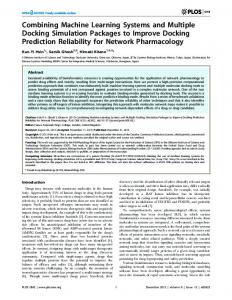
Friedman test at p = 0.05. Furthermore, by performing a series of Wilcoxon tests it was confirmed that AWEC increases (pC = 0.002) while AWED deteriorates (pD = 0.002) the accuracy of AWE. Looking at the results of AUE and its modifications we can see trends slightly different than those observed in AWE. The AUEW modification improves classification accuracy much more than AWEW but at higher processing costs. As AUEW updates existing component classifiers it can grow larger component Hoeffding trees, which require more time to test on a window of examples. Thus, the windowing technique is much more time consuming when used to modify AUE than it was on AWE. The additional incremental classifier, present in AUEC , allows to improve AUE’s accuracy on fast changing datasets such as TreeSR , CovType, Poker, and Power, but does not seem to be so useful on slower changing data. This is probably the effect of using a static (maximum) weight for the incremental candidate; in AWE which uses a linear weighting function it had a stronger impact than in AUE which uses a nonlinear quality measure (the difference between using a linear and nonlinear function will be discussed in Section 5.3). Nevertheless, the use of an additional incremental component gives comparable or better accuracy than the original AUE at very small time and memory costs. Finally, the use of a drift detector with AUE proves more rewarding than its addition to AWE. Since, in contrast to AWE, AUE’s components can be incrementally updated after a drift is detected, AUED manages to build strong component classifiers while AWE is left with weak learners after each drift. This seems to show that when combined with periodical incremental component updates a drift detector can enhance sudden drift reactions without degrading performance on gradual changes. As Table 2 shows, accuracies of AUE and its modifications are generally higher than AWE’s which could also be caused by incremental updating of component classifiers. Concerning classification accuracies of the modifications of AUE, the null hypothesis of the Friedman test can be rejected at p = 0.05, while the Wilcoxon test shows that AUEW and AUED significantly increase (pW = 0.001, pD = 0.01) the accuracy of AUE. According to the presented results, online component reweighting is the best transformation strategy in terms of accuracy. Unfortunately, it is also the most costly strategy in terms of processing time. Additionally, we have noticed that elements of incremental learning also improve classification accuracy. These findings were our motivation for creating an online ensemble, which uses incremental base learners and performs online component reweighting, but without additional processing costs. 5.3. Analysis of OAUE components As in block-based ensembles the block size is a parameter which largely influences the accuracy of the ensemble [35], we decided to verify the impact of using different block (and simultaneously window) sizes d for calculating the mean square error (M SEit , M SErt ) in OAUE. Table 5 presents the average prequential accuracy of OAUE on different datasets while using d ∈ [500; 2000]. Additionally, in Figure 1 we present three box plots summarizing the differences in accuracy, memory usage, and testing time of OAUE for different window sizes. The plots were created by, first calculating the mean performance value on each dataset over all window sizes, and later calculating and plotting the differences between the mean and the value obtained for a certain d. For example, for the Airlines dataset the mean value of average accuracies for all d ∈ [500; 2000] is 66.83%, therefore, the deviation for OAUE with d = 500, which has an average accuracy on Airlines equal 67.50, is +1.00%. Analyzing the values in Table 5, one can see that differences in each row are small and no global dependency upon d can be seen. Furthermore, the box plot in Figure 1(a) shows that most values are within 1% from the mean value on each dataset. Conversely, clear tendencies are visible on the plots of time and memory usage in Figures 1(b) and (c). The larger the window size, the longer and more memory consuming the classification. This dependency is an effect of creating each new classifier using d examples. When d grows, so does each candidate classifier, which means higher time and memory requirements. Performing a Friedman test on the calculated deviations for d ∈ [500; 2000] we obtain FFAcc = 2.183, FFM em = 34.594, and FFT ime = 3.857 for accuracy, memory usage, and evaluation time, respectively. As the critical value for α = 0.05 is 2.201, we reject the null-hypothesis for memory and time, but not for accuracy. According to the Friedman test, we can state that there is a difference in average processing time and memory usage for different values of d, but concerning accuracy there is no significant difference. As 14


Table 5: Average classification accuracy [%] of OAUE using different window sizes d

Window size


500

750

1000

1250

1500

1750

2000

67.50 90.07 90.55 89.05 53.40 51.54 80.24 81.54 15.73 96.78 96.69 88.95 89.41 46.23 84.34 83.86

66.93 90.85 90.43 89.04 53.40 51.48 80.23 87.92 15.58 97.59 97.27 88.85 89.32 46.05 85.25 84.75

67.03 90.91 90.42 88.94 53.38 51.40 80.23 88.87 15.54 97.83 97.38 88.81 89.31 45.86 85.47 84.85

67.12 91.08 90.26 89.00 53.24 51.39 80.20 90.18 15.34 97.84 97.46 88.79 89.28 45.21 85.58 84.87

66.72 91.43 90.30 88.98 52.65 51.35 80.20 90.81 15.27 97.96 97.56 88.70 89.23 44.39 85.53 84.86

66.33 91.51 90.24 88.92 52.40 51.27 80.20 92.01 15.23 98.00 97.53 88.67 89.22 43.66 85.50 84.73

66.23 91.58 90.19 88.97 52.38 51.28 80.17 92.65 14.87 97.90 97.43 88.62 89.15 43.28 85.49 84.66

(b) 6 %

150 % deviation from average memory usage

deviation from average prequential accuracy

(a) 4 % 2 % 0 % -2 % -4 % -6 % -8 %

500

750

1000 1250 1500 window size

(c)

1750

100 %

50 %

0 %

-50 %

-100 %

2000

500

750

1000 1250 1500 window size

1750

2000

deviation from average testing time

200 % 150 % 100 % 50 % 0 % -50 %

-100 %

500

750

1000 1250 1500 window size

1750

2000

Figure 1: Box plot of average prequential accuracy (a), memory usage (b), and testing time (c) for window sizes d ∈ [500; 2000]. The depicted values are the percentage deviation from the average on each dataset.

15


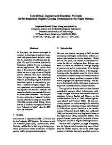
there is no strong dependency upon d in terms of accuracy, but time and memory are proportional, we decided to use d = 1000 as the value with least outliers and relatively low time and memory consumption. Apart from studying the influence of d, we performed another analysis concerning the impact of using different functions for weighting OAUE’s components. The experiments involved calculating average 1 t prequential accuracies for all test datasets using a nonlinear (wN L = M SErt +M SEit +ǫ ) and linear function t (wL = max{M SErt − M SEit , ǫ}). The results, omitted due to space limitations, showed that both functions performed almost identically on most datasets, with the linear function performing slightly better on datasets with very frequent changes and the nonlinear function being more accurate on datasets with noise and longer periods of stability. This dependency can be explained by analyzing component weights during a concept drift. A practical example of such a situation is depicted in Figure 2 were proportional weight t t values of ten components are depicted for OAUE using wN L (a) and wL (b). Nonlinear weighting function

(b)

Linear weighting function

100

100

90

90 component classifiers’ weights

component classifiers’ weights

(a)

80 70 60 50 40 30 20 10 0

80 70 60 50 40 30 20 10

14000

14200

14400 14600 timestamp

14800

0

15000

14000

14200

14400 14600 timestamp

14800

15000

Figure 2: Percentage component weight proportions of OAUE with a nonlinear weighting function (a) and OAUE with a linear weighting function (b)

As Figure 2 shows, compared with the nonlinear function, the linear function introduces larger proportional weight changes after each example. This can have the effect of faster reactions to changes, but means t that using wL the algorithm is more sensitive to noise. We performed a Wilcoxon signed rank test to comt t pare the accuracy of OAUE using wN L and wL . For α = 0.05, we were unable to reject the null-hypothesis t t and, therefore, we cannot see differences in using wN L or wL . In the comparative study presented below, we tested OAUE with the nonlinear function, as presented in Section 4. However, it is worth noting that using the presented linear function would yield a practically identical comparison with identical ranks for the Friedman test presented in Table 9. 5.4. Comparison of OAUE and other ensembles To evaluate the OAUE algorithm, we performed an experimental comparison involving four online ensembles: Online Bagging (Bag), Leveraging Bagging (Lev), the Dynamic Weighted Majority (DWM), and the Adaptive Classifier Ensemble (ACE). Online Bagging and Leveraging Bagging were chosen as strong representatives of online ensembles, DWM was selected because it periodically evaluates an ensemble and incrementally changes component weights, and ACE represents a processing scheme with a drift detector similar to the third of the proposed modification strategies. It is worth pointing out that ACE is an algorithm that was ported and not originally written for the MOA framework. This means that ACE used different base classes and its time and memory usage measured by MOA are not fully comparable with the remaining algorithms. Additionally, on the Wave, WaveM , and PAKDD datasets which contain a large number of attributes, ACE exceeded available memory and was unable to process the entire stream, while on other datasets ACE showcased very low memory usage. This only confirms that the memory usage calculated by MOA for ACE was underestimated and, therefore, we do not present memory usage of ACE. Average prequential accuracy, memory usage, and processing time for all algorithms is given in Tables 6-8. 16


Table 6: Average prequential classification accuracies [%]


ACE

DWM

Lev

Bag

OAUE

64.89 69.60 84.28 79.59 46.75 39.88 79.83 18.57 84.62 83.78 85.91 86.00 43.20 -

64.98 89.87 89.94 88.48 53.34 51.48 80.24 91.29 15.45 96.00 95.49 88.39 89.15 42.48 84.02 83.76

62.84 92.11 88.49 85.43 51.31 49.98 79.85 97.67 16.84 98.22 97.79 89.00 89.26 47.88 83.99 83.46

64.24 88.84 89.54 88.35 53.33 51.50 80.22 76.92 15.96 97.87 97.54 88.36 88.94 48.77 85.51 84.95

67.02 90.98 90.43 88.95 53.40 51.48 80.23 88.89 15.73 97.87 97.42 88.83 89.33 46.04 85.50 84.90

Additionally, we generated graphical plots for each dataset depicting the algorithms’ performance in terms of processing time, memory usage, and classification accuracy. Such graphical plots are a common way of examining the dynamics of a given classifier, in particular, its reactions to concept drift [11, 2]. Due to space limitations we will only analyze the most interesting accuracy and memory plots, which highlight characteristic features of the studied algorithms. 96 %

160 MB

94 %

DWM Lev Bag OAUE

140 MB

92 % 120 MB

90 %

100 MB Memory

Accuracy

88 % 86 % 84 %

80 MB 60 MB

82 % 40 MB

80 % ACE DWM Lev Bag OAUE

78 % 76 % 0

100 k 200 k 300 k 400 k 500 k 600 k 700 k 800 k 900 k

20 MB

1M

Processed instances

0 B 0

100 k 200 k 300 k 400 k 500 k 600 k 700 k 800 k 900 k

1M

Processed instances

Figure 4: Memory usage on the HyperF dataset

Figure 3: Prequential accuracy on the HyperF dataset

Figures 3 and 4 present the prequential accuracy and memory usage of the analyzed algorithms on the HyperF dataset, which contains fast incremental drift. The two best performing algorithms for this dataset were OAUE and DWM, which seem to react better to incremental changes than ACE, Lev, and Bag. The characteristic feature of DWM and OAUE is that they periodically change ensemble members, while the remaining three algorithms do that only when drift is detected. Similar behavior was observed in accuracy plots for the HyperS dataset, which contains a slow incremental drift. Looking at the memory plot in Figure 4, we can see that Lev requires much more memory than the remaining algorithms, Bag is second, while OAUE and DWM are the least memory expensive. This observation was consistent among most 17


Table 8: Algorithm testing time per d = 1000 examples [s]

Table 7: Average memory usage [MB]

ACE DWM Airlines CovType HyperF HyperS LEDM LEDN D PAKDD Poker Power RBFB RBFGR SEAG SEAS TreeSR Wave WaveM

0.30 -

Lev

Bag OAUE

86.26 63.73 60.27 8.27 6.75 1.19 4.37 63.41 7.19 4.24 110.11 6.31 0.61 1.76 2.56 0.41 0.98 1.32 3.16 38.26 6.24 2.25 4.62 0.17 0.09 0.11 0.11 6.36 60.21 13.07 6.22 52.94 13.15 1.73 31.05 4.06 1.32 67.33 7.32 1.81 3.75 1.10 6.18 480.29 69.71 6.42 190.03 26.16

89.90 3.09 3.23 2.87 0.32 0.32 3.39 2.18 0.18 8.03 11.06 1.45 2.66 2.28 50.63 12.29


ACE DWM

Lev

2.50 0.49 0.21 0.20 0.14 0.16 0.28 0.10 0.11 0.30 0.31 0.08 0.07 0.17 0.48 0.46

11.20 2.84 3.90 9.16 0.75 0.27 9.83 1.29 0.24 11.36 7.79 5.97 7.94 0.62 33.65 33.46

0.04 0.22 0.25 0.26 0.09 0.08 0.03 0.19 0.62 0.61 0.05 0.04 0.25 -

Bag OAUE 2.64 0.35 0.89 0.38 0.21 0.18 0.85 0.06 0.15 0.75 0.86 0.23 0.48 0.17 5.04 1.63

4.22 0.40 0.22 0.20 0.15 0.15 1.01 0.18 0.12 0.59 0.70 0.09 0.14 0.61 2.97 1.05

memory plots. It is also worth noticing that OAUE is one of the fastest of the analyzed algorithms and, in contrast to the analyzed online evaluation strategy from Section 3.2, does not introduce any additional processing cost compared to its block-based predecessor AUE. For streams with gradual drifts (RBFGR and SEAG ) the best performing algorithm is Lev, with OAUE and Bag being close second. However, Lev is also the slowest and most memory consuming algorithm on these datasets, requiring on an average 13 times more memory and 38 times more processing time than OAUE. Figure 5 presents the accuracies of the analyzed algorithms on the RBFGR dataset. Gradual drifts created around examples number 125, 250, 375, 500k have the worst impact on DWM and ACE. ACE uses static batch learners and, therefore, is not capable of reacting quickly to gradual changes. DWM on the other hand is probably performing slightly worse because it uses a penalty function which strongly diminishes component weights during prolonged drifts. 100 %

Accuracy

95 %

90 %

85 %

80 %

75 % 0

ACE DWM Lev Bag OAUE

100 k 200 k 300 k 400 k 500 k 600 k 700 k 800 k 900 k

1M

Processed instances

Figure 5: Prequential accuracy on the RBFGR dataset

Depending on the frequency of drifts, the best performing algorithms for streams with sudden changes were OAUE and Bag. For rare abrupt changes, such as in the SEAS dataset, OAUE suffered the smallest 18


accuracy drops. However, for very fast changes present in the TreeSR stream, algorithms with drift detectors, such as Lev and Bag, perform much better in terms of accuracy. What is worth noting is that using OAUE with a linear weighting function (as presented in Section 5.3) would yield an accuracy of 49.68%, which would be the best result for this dataset. This shows that for very dynamic changes either drift detectors or very drastic component weight modifications are required to adapt in time. On datasets with no drift (LEDN D ), with drifting attribute values (Wave, WaveM ) or added noise (LEDM , RBFB ), OAUE, Bag, and DWM perform almost identically, with Lev and ACE being slightly less accurate. On real datasets, in terms of accuracy, there is no single best performing algorithm. On Poker Lev clearly outperforms all the other algorithms. On CovType, Lev is the most accurate followed by OAUE, while on PAKDD all the algorithms perform almost identically. On the other hand, OAUE is the most accurate on the Airlines dataset, while ACE is the best on Power. To conclude the analysis, we carried out statistical tests for comparing multiple classifiers over multiple datasets. We used the non-parametric Friedman test, for which the null-hypothesis is that there is no difference between the performance of all the tested algorithms. Moreover, in case of rejecting this nullhypothesis we use the Bonferroni-Dunn post-hoc test [9, 20] to verify whether the performance of OAUE is statistically different from the remaining algorithms. The average ranks of the analyzed algorithms are presented in Table 9 (the lower the rank the better). Table 9: Average algorithm ranks used in the Friedman tests

Accuracy Memory Testing time

ACE

DWM

Lev

Bag

OAUE

4.50 2.50

2.94 1.81 1.81

2.75 3.56 4.81

2.75 2.63 3.19

2.06 2.00 2.69

By using the Friedman test to verify the differences between accuracies, we obtain FFAcc = 7.248. As the critical value for comparing 5 algorithms over 16 datasets for α = 0.05 is 2.525, the null hypothesis can be rejected. Considering accuracies, OAUE provides the best average achieving usually 1st or 2nd rank on each dataset. To verify whether OAUE performs better than the remaining algorithms, we compute the critical difference chosen by the Bonferroni-Dunn test [9, 20] as CD = 1.396. This allows us to state that OAUE is significantly more accurate then ACE, but concerning the remaining algorithms the experimental data is not sufficient to reach such a conclusion. However, by performing additional one-tailed Wilcoxon signed rank tests for comparing pairs of classifiers, we can state that OAUE is more accurate than DWM with pDW M = 0.004. The p-value for stating that OAUE is more accurate than Bag and Lev are pBag = 0.089 and pLev = 0.163 respectively. Overall, the conducted experiments seem to support our observation that in terms of accuracy OAUE is not only comparable to other systems in the literature, but in most cases achieves better performance. Performing a similar analysis for memory usage and processing time we get FFM em = 6.793 and FFT ime = 15.476 respectively, which allows us to reject the null-hypothesis in both cases. Analyzing the CD and by performing Wilcoxon tests we can state that OAUE is significantly faster than Lev (pLev = 0.0002) and less memory consuming than Lev and Bag (pLev = 0.001, pBag = 0.022). 6. Conclusions In this paper, we studied the problem of integrating weighting mechanisms and periodical component evaluations, known from block ensembles, into online classifiers for mining concept drifting data streams. First, we analyzed which methods for transforming block-based ensembles into online learners are most promising in terms of classification accuracy and computational costs. We proposed three general transformation strategies: an online evaluation technique, the introduction of an incremental learner, and the use of a drift detector. Experimental evaluation of these strategies showed that incremental training combined with online component reweighting were most beneficial in terms of accuracy. However, the analyzed online 19


reweighting strategy, which used a sliding window of examples, suffered from high time and memory costs due to excessive processing of full examples. Based on these findings, we proposed a new incremental stream classifier, called Online Accuracy Updated Ensemble (OAUE), which trains and weights component classifiers with each incoming example. The main novelty of the OAUE algorithm is the proposal of a cost-effective component weighting function, which estimates a classifier’s error on a window of last seen instances in constant time and memory without the need of remembering past examples. We also carried out experimental studies analyzing the effect of using different window sizes and functions for evaluating component classifiers. The obtained results showed that the accuracy of the proposed algorithm did not change depending on the window size, but larger windows induced higher time and memory costs. Concerning different error-based weighting functions, we have found that linear functions performed better on fast drifting streams, but nonlinear functions were more robust to noise. Finally, we experimentally compared OAUE with four representative online ensembles: the Adaptive Classifier Ensemble, Dynamic Weighted Majority, Online Bagging, and Leveraging Bagging. The obtained results demonstrated that OAUE can offer high classification accuracy in online environments regardless of the existence or type of drift. OAUE provided best average classification accuracy out of all the tested algorithms and was among the least time and memory consuming. As future work, we plan to investigate the problem of introducing additional diversity to online component learning. Acknowledgement The authors are grateful to Dr. Kyosuke Nishida and Dr. Paulo Gon¸calves for sharing their implementations of the Adaptive Classifier Ensemble and Learn++.NSE algorithms. This work was partly supported by the Polish National Science Center under Grant No. DEC-2011/03/N/ST6/00360. References [1] A. Bifet, G. Holmes, R. Kirkby, B. Pfahringer, MOA: Massive Online Analysis, J. Mach. Learn. Res. 11 (2010) 1601–1604. [2] A. Bifet, G. Holmes, B. Pfahringer, Leveraging bagging for evolving data streams, in: ECML/PKDD (1), 2010, pp. 135–150. [3] A. Bifet, G. Holmes, B. Pfahringer, R. Kirkby, R. Gavald` a, New ensemble methods for evolving data streams, in: Proc. 15th ACM SIGKDD Int. Conf. Knowledge Discovery Data Mining, 2009, pp. 139–148. [4] A. Bifet, J. Read, B. Pfahringer, G. Holmes, I. Zliobaite, CD-MOA: Change detection framework for massive online analysis, in: Proc. of the 20th Int. Symposium on Intelligent Data Analysis (IDA’13), 2013. [5] D. Brzezinski, J. Stefanowski, Accuracy updated ensemble for data streams with concept drift, in: Proc. 6th HAIS Int. Conf. Hyb. Art. Intell. Syst., Part II, vol. 6679 of LNCS, Springer, 2011, pp. 155–163. [6] D. Brzezinski, J. Stefanowski, Reacting to different types of concept drift: The accuracy updated ensemble algorithm, IEEE Transactions on Neural Networks and Learning Systems 24 (7). [7] E. Cohen, M. J. Strauss, Maintaining time-decaying stream aggregates, J. Algorithms 59 (1) (2006) 19–36. [8] M. Deckert, Batch weighted ensemble for mining data streams with concept drift, in: Proc 20th ISMIS Int. Symp., vol. 6804 of LNCS, Springer, 2011, pp. 290–299. [9] J. Demsar, Statistical comparisons of classifiers over multiple data sets, J. Machine Learning Research 7 (2006) 1–30. [10] P. Domingos, G. Hulten, Mining high-speed data streams, in: Proc. 6th ACM SIGKDD Int. Conf. Knowl. Disc. Data Min., ACM Press, USA, 2000, pp. 71–80. [11] R. Elwell, R. Polikar, Incremental learning of concept drift in nonstationary environments, IEEE Trans. Neural Netw. 22 (10) (2011) 1517–1531. [12] W. Fan, Y. an Huang, H. Wang, P. S. Yu, Active mining of data streams, in: Proc. 4th SIAM Int. Conf. Data Mining, 2004, pp. 457–461. [13] A. Frank, A. Asuncion, UCI machine learning repository, http://archive.ics.uci.edu/ml (2010). URL http://archive.ics.uci.edu/ml [14] J. Gama, Knowledge Discovery from Data Streams, Chapman and Hall, 2010. [15] J. Gama, P. Medas, G. Castillo, P. Rodrigues, Learning with drift detection, in: Proc. 17th SBIA Brazilian Symp. Art. Intel., 2004, pp. 286–295. [16] J. Gama, R. Sebasti˜ ao, P. P. Rodrigues, On evaluating stream learning algorithms, Machine Learning 90 (3) (2013) 317–346. [17] S. Greco, R. Slowinski, I. Szczech, Properties of rule interestingness measures and alternative approaches to normalization of measures, Information Sciences 216 (2012) 1–16. [18] J. Han, Data Mining: Concepts and Techniques, Morgan Kaufmann Publishers Inc., San Francisco, CA, USA, 2005.

20


[19] G. Hulten, L. Spencer, P. Domingos, Mining time-changing data streams, in: Proc. 7th ACM SIGKDD Int. Conf. Knowledge Discovery Data Mining, 2001, pp. 97–106. [20] N. Japkowicz, M. Shah, Evaluating Learning Algorithms: A Classification Perspective, Cambridge University Press, New York, NY, USA, 2011. [21] J. Z. Kolter, M. A. Maloof, Dynamic weighted majority: An ensemble method for drifting concepts, J. Mach. Learn. Res. 8 (2007) 2755–2790. [22] L. I. Kuncheva, Classifier ensembles for changing environments, in: Proc. 5th MCS Int. Workshop on Mult. Class. Syst., vol. 3077 of LNCS, Springer, 2004, pp. 1–15. [23] L. I. Kuncheva, Combining Pattern Classifiers: Methods and Algorithms, Wiley-Interscience, 2004. [24] L. I. Kuncheva, Classifier ensembles for detecting concept change in streaming data: Overview and perspectives, in: Proc. 2nd Workshop SUEMA 2008 (ECAI 2008), 2008, pp. 5–10. [25] N. Littlestone, M. K. Warmuth, The weighted majority algorithm, Inf. Comput. 108 (2) (1994) 212–261. [26] O. Maimon, L. Rokach (eds.), Data Mining and Knowledge Discovery Handbook, 2nd ed, Springer, 2010. [27] M. M. Masud, J. Gao, L. Khan, J. Han, B. M. Thuraisingham, A practical approach to classify evolving data streams: Training with limited amount of labeled data, in: ICDM, IEEE Computer Society, 2008, pp. 929–934. [28] L. L. Minku, A. P. White, X. Yao, The impact of diversity on online ensemble learning in the presence of concept drift, IEEE Trans. Knowl. Data Eng. 22 (5) (2010) 730–742. [29] L. L. Minku, X. Yao, DDD: A new ensemble approach for dealing with concept drift, IEEE Trans. Knowl. Data Eng. 24 (4) (2012) 619–633. [30] K. Nishida, K. Yamauchi, T. Omori, ACE: Adaptive classifiers-ensemble system for concept-drifting environments, in: Proc. 6th Int. Workshop Multiple Classifier Systems, vol. 3541 of LNCS, Springer, 2005, pp. 176–185. [31] N. C. Oza, S. J. Russell, Experimental comparisons of online and batch versions of bagging and boosting, in: Proc. 7th ACM SIGKDD Int. Conf. Knowl. Disc. Data Min., ACM Press, New York, NY, USA, 2001, pp. 359–364. [32] Pakdd 2009 data mining competition. URL http://sede.neurotech.com.br:443/PAKDD2009/ [33] W. N. Street, Y. Kim, A streaming ensemble algorithm (SEA) for large-scale classification, in: Proc. 7th ACM SIGKDD Int. Conf. Knowl. Disc. Data Min., ACM Press, New York, NY, USA, 2001, pp. 377–382. [34] A. Tsymbal, The problem of concept drift: definitions and related works, Tech. rep., Dept. Comput. Sci., Trinity College Dublin (2004). [35] H. Wang, W. Fan, P. Yu, J. Han, Mining concept-drifting data streams using ensemble classifiers, in: Proc. 9th ACM SIGKDD Int. Conf. Knowl. Disc. Data Min., ACM Press, USA, 2003, pp. 226–235. [36] Y. Yao, L. Feng, F. Chen, Concept drift visualization, Journal of Information and Computational Science 10 (10) (2013) 3021–3029. [37] S. Yoshida, K. Hatano, E. Takimoto, M. Takeda, Adaptive online prediction using weighted windows, IEICE Transactions 94-D (10) (2011) 1917–1923. [38] I. Zliobaite, Combining time and space similarity for small size learning under concept drift, in: Proc 18th ISMIS Int. Symp., 2009, pp. 412–421. [39] I. Zliobaite, A. Bifet, B. Pfahringer, G. Holmes, Active learning with evolving streaming data, in: D. Gunopulos, T. Hofmann, D. Malerba, M. Vazirgiannis (eds.), ECML/PKDD (3), vol. 6913 of Lecture Notes in Computer Science, Springer, 2011, pp. 597–612.

21

Combining block-based and online methods in learning ensembles ...

Combining block-based and online methods in learning ensembles ...

Suggest Documents

A comparison of methods for learning and combining evidence from ...

Combining Lexicon-based and Learning-based Methods for Twitter ...

Combining Methods in Legal Research

Combining Qualitative and Quantitative Methods in

Combining and Comparing Cluster Methods in a

Combining Qualitative and Quantitative Methods in Information ...

Combining qualitative and quantitative methods in ...

Combining qualitative and quantitative methods in

Combining Qualitative and Quantitative Methods In Environmental

Corpus triangulation: combining data and methods in

Neural Network Ensembles in Reinforcement Learning

Predictive learning via rule ensembles

Combining Machine Learning Systems and

Online Learning of Portfolio Ensembles with Sector Exposure ...

Measures of Diversity in Classifier Ensembles and ... - Machine Learning

Combining Classroom-Based Learning and Online ... - Archive EduTice

Combining Linguistic and Statistical Methods for ... - People.csail.mit.edu

METHODS & TECHNIQUES Combining forces and kinematics for ...

Combining Revealed and Stated Preference Methods for

Combining Metaheuristics and Exact Methods to ...

Combining and Benchmarking Methods of Foetal ...

Combining Stochastic Optimization and Numerical Methods-Software ...

Combining DFT and many-body methods to

Combining Formal Methods and Functional Strategies ... - CiteSeerX