xRT (ARM). 1.18. 1.35. Table 1. Baseline Results. In PocketSphinx, mixture weights are stored as logarith- mic values with a small base (typically 1.0001) which ...
COMBINING MIXTURE WEIGHT PRUNING AND QUANTIZATION FOR SMALL-FOOTPRINT SPEECH RECOGNITION David Huggins-Daines and Alexander I. Rudnicky Carnegie Mellon University Language Technologies Institute Pittsburgh, PA, USA ABSTRACT Semi-continuous acoustic models, where the output distributions for all Hidden Markov Model states share a common codebook of Gaussian density functions, are a well-known and proven technique for reducing computation in automatic speech recognition. However, the size of the parameter files, and thus their memory footprint at runtime, can be very large. We demonstrate how non-linear quantization can be combined with a mixture weight distribution pruning technique to halve the size of the models with minimal performance overhead and no increase in error rate. Index Terms— Speech recognition, Quantization, Data compression 1. INTRODUCTION In large-vocabulary continuous speech recognition, the computational load is typically evenly divided between acoustic model evaluation and large-vocabulary search. The speed of the recognizer is directly proportional to, on the one hand, the number of basic acoustic models (typically Gaussian or Laplacian densities) which are evaluated per frame of input, and on the other hand, the number of arcs (word or phone models) in the search graph which are active per frame. A well-known way to reduce the number of Gaussian densities to be evaluated is to share a common codebook of densities between some or all states in the acoustic model. If a single codebook is shared between all states, this is known as a semi-continauous acoustic model [1]. It is also common to split the acoustic feature space into multiple independent streams, with a separate codebook for each stream. In the PocketSphinx system [2], four codebooks of 256 Gaussians, modeling 12 MFCC coefficients, their first and second time derivatives, and the power coefficients, are shared between all states of the acoustic model. Each tied output distribution, or senone, is represented by four arrays of 256 mixture weights, corresponding to the 1024 shared Gaussians. Therefore, although the amount of Gaussian computation is greatly reduced, the mixture weight parameter arrays can be quite large, containing 1024 parameters for each senone in
978-1-4244-2354-5/09/$25.00 ©2009 IEEE
4189
the model. Furthermore, to compensate for the small number of Gaussian densities, it is common to use a large number of senones in order to take advantage of large training data sets. Despite the size of the mixture weight arrays, in our experience, evaluation of semi-continuous models is more efficient than evaluation of similar types of compact acoustic models, such as subspace distribution clustered HMMs [3]. There are two reasons for this. The first is that, as is typically the case in mixture models, the vast majority of the probability mass for any given observation falls on a small number of Gaussians in each codebook. Since the codebook of Gaussians itself is relatively small, most of the work in evaluating a set of semicontinuous models lies in the calculation of mixture densities. We can save a substantial amount of computation by using only the top N Gaussians in calculating mixture densities, for some small N , usually 4 in our system. This is possible due to the stream independence property of semi-continuous models. As shown in Equation 1, the codebook density is contained inside a summation over all weighted, normalized components for a given feature stream. Therefore, if a density has been skipped and is presumed to be zero, it simply does not contribute to the overall mixture density. PSC (o|qi ) =
�� j
k
N (o; μijk , Σijk ) wijk � � N (o; μij� , Σij� )
(1)
By contrast, in a subspace-distribution model, shown in Equation 2, the codebook densities are contained inside a product over feature streams for a given mixture component. A missing density here forces the entire component density to zero. Also, since mixture densities are typically computed in logarithmic form, the “sum” operation is considerably more expensive than the “product” operation, and so there is no real advantage to skipping densities. PSDC (o|qi ) =
� k
wik
�
N (o; μijk , Σijk )
(2)
j
The second reason for the efficiency of semi-continuous models is that the direct mapping of GMM components to
ICASSP 2009
codebook Gaussians allows the mixture weights to be arranged in component-major order in memory. Since only a few components are used in calculating scores, memory accesses to the mixture weight array are localized to the contiguous regions corresponding to these components. When the mixture weights are stored in senone-major order, the access pattern is much sparser, leading to frequent cache misses. In this paper, we examine the effect of combining mixture weight pruning and compression in order to reduce the memory footprint of semi-continuous models without compromising their efficiency of evaluation.
3. MIXTURE WEIGHT PRUNING In general, for any given senone, a few components comprise the majority of the a priori probability mass in the mixture weight distribution. That is, the average entropy of the mixture weight distribution is quite low. It was shown in [5] that the stream independence property allows us to exploit this fact by removing “irrelevant” mixture weights from the distribution. This is done by taking the average perplexity of the unpruned mixture weight distributions and computing a scaling factor between it and a desired average “target” number t of non-zero weights per senone. This factor is applied to the perplexity of each mixture weight distribution wi and the resulting top ni , up to a minimum value k, values are retained:
2. EXPERIMENTAL SETUP
ni = max(k,
For our experiments in this paper, we used the Wall Street Journal corpus of read speech [4]. Semi-continuous acoustic models were trained on the full set of training data, including the speaker independent and dependent sets and the “spontaneous” training data, for a total of approximately 190 hours of speech. The traning data was downsampled to 8kHz to match the input capabilities of typical mobile devices. We used the PocketSphinx decoder, in single-pass recognition mode, with acoustic features as described above. The language model was the Lincoln Labs 5000-word closed vocabulary trigram model with non-vocalized punctuation. Baseline results for 5000 and 10000 senone models on the 5000-word vocabulary November ’92 development and test sets are shown in Table 1. The real-time factors reported are for the development set, and do not include acoustic feature extraction. The “x64” system is an AMD Opteron 852 running at 2.6 GHz, while the “ARM” system is a Nokia N800 tablet using a TI OMAP 2420 running at 400MHz. Senones %WER (devel) %WER (test) xRT (x64) xRT (ARM)
5000 11.85 9.73 0.07 1.18
10000 11.01 9.13 0.08 1.35
Table 1. Baseline Results In PocketSphinx, mixture weights are stored as logarithmic values with a small base (typically 1.0001) which are converted to integers, negated, and linearly quantized such that the sum of a log mixture weight and log acoustic density never exceeds 255. This allows the “addition” operation in logarithmic space to be done using a small lookup table indexed by the difference between two values. The normalization of Gaussian densities, as shown in Equation 1, is very important to this implementation, as it reduces their dynamic range.
1 N
�N
i=0
t pplx(wi )
pplx(wi ))
(3)
This results in a substantial improvement in runtime performance, as shown in Table 2 for the development set. The performance gain with pruned mixtures does not come from more efficient mixture density calculation, but rather from an effect on the distribution of acoustic scores which causes outlier models to be removed from search earlier. This effect is complimentary to beam pruning, as shown in the timeaccuracy curves in Figure 1. Target t 32 %WER (10000) 13.17 xRT (10000) 0.04 %WER (5000) 15.24 xRT (5000) 0.03 xRT (5000, ARM)
48 12.13 0.05 13.45 0.04
64 11.35 0.06 12.27 0.05
96 11.07 0.07 11.72 0.05 1.03
128 11.15 0.08 11.68 0.06
Table 2. Mixture Weight Pruning (Nov ’92 devel 5k) The problem with mixture weight pruning is that, in order to preserve this improvement in performance, it is necessary to preserve the size and structure of the mixture weight array. That is, the “irrelevant” mixture weights are not actually removed from the in-memory representation, but simply set to zero (or, to be precise, the maximum allowable value, since they are stored as negative log quantities). The componentmajor access pattern described in Section 1, which is crucial to fast evaluation, requires that all mixture weights for a given Gaussian be stored contiguously in memory, and therefore we cannot simply store the non-zero mixture weights for each senone, though there may only be a few of them. 4. MIXTURE WEIGHT QUANTIZATION Another option for compressing the mixture weight arrays, implemented in the Microsoft Whisper system [6], which was derived from the Sphinx-II system [7], which was succeeded by PocketSphinx, is to use run-length encoding on the rows
4190
Codewords %WER (10000) (96 mixtures) xRT (10000) (96 mixtures) %WER (5000) (96 mixtures) xRT (5000) (96 mixtures)
280
48 mixtures 64 mixtures 96 mixtures 256 mixtures
260
seconds CPU time
240 220 200 180
4 17.40 14.23 0.18 0.11 19.50 13.89 0.17 0.08
8 11.28 11.04 0.09 0.07 13.25 12.28 0.09 0.06
16 11.09 11.72 0.08 0.07 12.52 11.31 0.08 0.06
32 11.01 11.17 0.08 0.07 11.76 11.75 0.07 0.06
64 11.22 11.19 0.08 0.07 11.66 11.79 0.07 0.05
Table 3. Mixture Weight Quantization, Nov ’92 devel 5k
160 140
5. MIXTURE WEIGHT COMPRESSION
120 100 10
12
14
16
18
20
22
24
26
% WER
Fig. 1. Time-Accuracy of Pruned Models (Nov ’92 devel 5k, 10000 senones) of the component-major mixture weight arrays. For this to be an effective form of compression, it must be combined with quantization of the mixture weight values. As noted in Section 2, the log-mixture weights in PocketSphinx are already stored in a linearly quantized form. However, this format was chosen specifically to make the log-addition operation computationally efficient, and is not storage efficient. Although the range of the mixture weights is 0 to 159, they are stored as single bytes. As well, contrary to [6], we found that there were very few runs of specific values long enough to achieve significant space savings with RLE. For this reason, we investigated non-linear quantization of the mixture weight values. Using a Lloyd-Max quantizer, we constructed codebooks from the original, unquantized log mixture weights, excluding the “zero” probability values, which were represented by a fixed codeword. These codebooks were then linearly quantized to the same 8-bit representation required by the log-addition code. To investigate the effect on accuracy, we ran experiments where the original mixture weights were simply replaced with the nearest codeword. As shown in Table 3, there is little effect on accuracy when using as few as 8 codewords, and no effect on speed when using as few as 16 codewords. As well, when mixture weight pruning is applied before quantization, there is a smaller penalty in accuracy and speed. The slowdown incurred with 8 codewords is similar to the slowdown we experience when raising the mixture weight floor, as described in [5]. Namely, it flattens the distribution of acoustic scores, causing outlier models to be kept active in search longer than necessary. The same pattern can be observed in the test set; in fact, the performance of pruned and quantized models (10000 senones, 96 mixtures and 16 codewords) is equal to the baseline on the test set (9.11% WER versus 9.13%).
Since the performance of the recognizer using 16 codewords is indistinguishable from that using the original mixture weights, this allows us to immediately cut the size of the mixture weight array in half by using a fixed width 4-bit encoding for the codeword indices. In addition, the scaled acoustic densities for the top N Gaussians can now be precomputed since there are only 16N distinct values, each of which occupies a single byte. Senones Uncompressed 4-bit encoded RLE (unpruned) RLE (96 mixtures)
5000 5,345,864 2,673,239 4,005,919 2,244,351
10000 10,465,920 5,233,240 7,293,083 4,202,484
Table 4. Compressed Mixture Weight File Sizes (bytes) We also implemented a run-length encoding scheme, using the top 4 bits of each byte in the mixture weight array to store the run length, and the low 4 bits to store the codeword index. As shown in Table 4, we found that this was only effective by comparison with the fixed width encoding when mixture weight pruning was first applied. The run-length encoding scheme also incurred a significant overhead in CPU time, particularly on the ARM platform, as shown in Table 5. This is most likely because it is necessary to scan the entire mixture weight array to obtain codeword indices, even if the set of active senones is sparse. This is a particular problem for the ARM platform which has only a single 16 KiB data cache and a much slower path to main memory. Conversely, the 4-bit encoding consistently decreases performance by approximately 20% on x64, but behaves inconsistenly on ARM, decreasing performance by only 2% in the best case and 26% in the worst case. This is most likely due to better branch prediction on the x64 platform, since the extraction of the 4-bit codeword IDs from the mixture weight array uses a parity test and branch to determine which half-byte to extract. An alternative method is to implement the half-byte indexing using a variable shift count calculated from the parity bit. This proved to be less efficient on x64, and roughly
4191
Platform Senones unpruned 4-bit RLE 96 mixtures 4-bit RLE
5000 0.07 0.10 0.11 0.05 0.06 0.07
x64 10000 0.08 0.10 0.13 0.07 0.09 0.11
ARM 5000 10000 1.18 1.35 1.49 1.39 1.71 1.87 1.03 1.20 1.05 1.35 1.21 1.66
to offset any benefits resulting from the reduced memory footprint. This overhead is likely to be greater on embedded platforms due to their simpler and lower-performing memory hierarchies. 7. REFERENCES
Table 5. Performance of Compressed Mixture Weights (xRT) the same on ARM. Another efficient way to implement 4-bit encoding is to activate and compute senones in even/odd pairs. Although this leads to more senone scores being computed per frame, the reduced overhead for indexing and unpacking half-byte values causes it to be slightly faster on x64. Since the senone score computation is more memory-bound on ARM, it has little to no effect on that platform.
[1] X. D. Huang, Semi-continuous Hidden Markov Models for Speech Recognition, Ph.D. thesis, University of Edinburgh, 1989. [2] D. Huggins-Daines, M. Kumar, A. Chan, A. Black, M. Ravishankar, and A. Rudnicky, “PocketSphinx: A free, real-time continuous speech recognition system for hand-held devices,” in Proceedings of ICASSP 2006, Toulouse, France, 2006. [3] E. Bocchieri and B. Mak, “Subspace distribution clustering hidden markov model,” IEEE Transactions on Speech and Audio Processing, vol. 9, no. 3, pp. 264–275, 2001. [4] D. Paul and J. Baker, “The design for the Wall Street Journal based CSR corpus,” in Proceedings of the ACL workshop on Speech and Natural Language, 1992.
6. CONCLUSIONS AND FUTURE WORK The combination of mixture weight distribution pruning and non-linear quantization of mixture weight parameters can reduce the memory and storage footprint of the decoder by several megabytes for a typical acoustic model. While quantization alone incurs a significant performance overhead, this can be reduced or eliminated by combining it with pruning. In addition, the run-length encoding scheme proposed in [6] achieves much better compression and performance when combined with mixture weight pruning. Overall, the combination of a fixed 4-bit coding scheme and mixture weight pruning was the most successful, achieving a 2.6 MB savings in model size and memory footprint with a negligible impact on performance on the ARM platform (1.05 xRT versus 1.03 xRT for the pruned, uncompressed model and 1.18 xRT for the baseline model). As well, the error rate for the 5000-senone pruned and compressed model is actually lower on the development set than the baseline model (11.31% versus 11.85%). This, or a scheme similar to it, will be implemented in future versions of the PocketSphinx speech recognition system and released as open source code through the CMU Sphinx project (http://cmusphinx.org). Since the distribution of mixture weight codewords is far from uniform, it may be possible in the future to achieve better compression using Huffman coding or some other variable-width code. This is particularly promising with pruned mixture weight distributions since the effect of pruning is to decrease the entropy of these distributions, and more so their quantized representations. However, as with run-length encoding, the additional overhead incurred by scanning the compressed mixture arrays at runtime is likely
4192
[5] D. Huggins-Daines and A. Rudnicky, “Mixture pruning and roughening for scalable acoustic models,” in Proceedings of ACL Workshop on Mobile Language Technologies, Columbus, OH, USA, 2008. [6] X. D. Huang, A. Acero, F. Alleva, M. Hwang, L. Jiang, and M. Mahajan, “From Sphinx-II to Whisper: Making speech recognition usable,” in Automatic Speech and Speaker Recognition: Advanced Topics, pp. 481–508. Kluwer, 1996. [7] X. D. Huang, F. Alleva, H. Hon, M. Hwang, and R. Rosenfeld, “The Sphinx-II speech recognition system: an overview,” Computer Speech and Language, vol. 7, no. 2, pp. 137–148, 1993.