Community Detecting By Signaling on Complex Networks

arXiv:0710.5441v1 [physics.soc-ph] 29 Oct 2007

Community Detecting By Signaling on Complex Networks Yanqing Hu, Menghui Li, Peng Zhang, Ying Fan, Zengru Di∗ Department of Systems Science, School of Management Center for Complexity Research Beijing Normal University, Beijing 100875, P.R.China February 2, 2008

Abstract Based on signaling process on complex networks, a method for identification community structure is proposed. For a network with n nodes, every node is assumed to be a system which can send, receive, and record signals. Each node is taken as the initial signal source once to inspire the whole network by exciting its neighbors and then the source node is endowed a nd vector which recording the effects of signaling process. So by this process, the topological relationship of nodes on networks could be transferred into the geometrical structure of vectors in nd Euclidian space. Then the best partition of groups is determined by F -statistic and the final community structure is given by Fuzzy C-means clustering method (FCM). This method can detect community structure both in unweighted and weighted networks without any extra parameters. It has been applied to ad hoc networks and some real networks including Zachary Karate Club network and football team network. The results are compared with that of other approaches and the evidence indicates that the algorithm based on signaling process is effective.

Keyword: Complex network, Community Structure, Signaling Algorithm, FCM PACS: 89.75.Hc, 89.75.Fb, 89.65.-s

1

Introduction

The study of complex networks has received an enormous amount of attention[1, 2, 3] from the scientific community in recent years. Physicists in particular have become interested in the study of networks describing the topologies of wide variety of systems, such as the world wide web[4], social and communication networks[5, 6], biochemical networks and many more[7]. One such problem is the analysis of community structure found in many networks. ∗ Author

for correspondence: [email protected]

1

Distinct communities or modules within networks can loosely be defined as subsets of nodes which are more densely linked, when compared to the rest of the network[8, 9]. Such communities have been observed, using some of the methods, in many different contexts, including metabolic networks, banking networks and most notably social networks. As a result, the problem of identification of communities has been the focus of many recent efforts. Community detection in large networks is potentially very useful. Nodes belonging to a tight-knit community are more than likely to have other properties in common. Besides, these communities may probably be functional groups, which provide us valuable reference to our study in many other fields. In recent studies, the scientists have designed many different algorithms[8, 9, 10, 11, 12, 13, 14, 15, 16, 17, 18, 19, 20, 21, 22, 23, 24](see [12] as a review) to detect the community structures. These algorithms can be divided into categories. Some algorithms are designed according to maximal modularity Q. Some are designed based on topology structures (betweenness, degree, or clustering coefficient). The last is designed according to the dynamical properties of the network. Communities within networks can be defined as subsets of nodes which are more densely linked, when compared to the rest of the network. Modularity Q is an index advanced by Newman and Grivan[25] as a measurement for the community structure. It gives a clear and precise definition of characteristics of the acknowledged community and have very successful application in practice. So it leads to many other algorithms brought forward to divide a community by maximizing Modularity Q. Unfortunately, maximizing Modularity Q has been proven a NPC problem[26], which makes it unable to work out the partition corresponding to maximal Q in a network which has lots nodes. Actually many algorithms for maximizing Q are usually heuristic algorithm. Besides, Modularity Q has been proven strictly that, as an index to measure the community structure, it tends to combine the little communities rather than identify them successfully in the networks with definite communities[27]. Though Modularity Q is proven to have the above-mentioned inherent defects, it is still the successful index to measure a network for the moment. Therefore, lots of work for detecting communities are dependent on the index Q. Among the algorithms based on network topology, we want to introduce briefly the spectral analysis method and GN algorithm[9]. GN algorithm was proposed by Grivan and Newman. It gives the division of network by remove links. The links with largest betweenness are removed one by one in order to split hierarchically the graph into community. But GN algorithm alone can only give the dendrogram concerning the network structure finally. It could not give the best partition directly. If we want to get the best partition we have to depend on Modularity Q or other indexes to work it out. While the principle of the spectral analysis method[29] is based on the theory of eigenvector of matrix. When a network is partitioned into two communities with the pre-fixed sizes, the best partition is to make the number of edges between the two communities being minimum. In fact, this problem is closely related to the eigenvector corresponding with the Fiedler eigenvector (the eigenvector correspond to second minimum eigenvalue) of Laplacian matrix of a network. Relatively speaking, spectral analysis method is the most math theory-based approach. But it’s still unable to get the best partition. Besides, it requires to know the sizes of the two sub-network beforehand. Although some methods are proposed to solve the two defects, like getting the best partition by using Q, ascertaining the sizes of the two sub-network by the sign of the elements of Fielder eigenvector and so on, the inherent defects of spectral analysis method have not been solved perfectly and completely yet.

2

There are still other algorithms based on the dynamics on networks, among which random walks[14] method and circuit approach method[17] will be briefly discussed here. In the random walks method, each node contains a walker initially. Then each walker will randomly choose a neighbor of the node it currently stand on to localize. This is a Markov process. After a period of time, the possibility will be higher that the walker reach another node belonging to the same community of the node the walker stood on at the beginning. And this possibility can be directly regarded as the possibility of pair of nodes in the same community and through it, a dendrogram can be got, then partition can be made by the aid of Modularity Q. When using random walk method to detect communities, it’s difficult to specify the optimum random-walking time. And the best partition is dependent on the external index Q usually. The principle of circuit approach method is to regard the edges of the network as the resistances, and add voltage to the adequate nodes of the network, then work out the voltage of each node by Kirchhoff’s law. Nodes with the similar voltages are regarded to exist in the same community more probably. At the same time, define the external indexes such as tolerance to realize the partition of the network. In this paper, we propose a new algorithm for identification communities based on signaling process on network. In this approach, every node is viewed as a system which can be inspired. It can send, receive, and record signals. In the initial, a node is selected as the source of signal. We give it an initial unit signal and other nodes with the signal of zero. Then the source node send the signal to its neighbors and itself first. Afterwards, the nodes with signals can also send signals to their neighbors and themselves. One thing should be mentioned in this signaling process is that the node can record the amount of signals it received, and at every time step, each node sends its present-owning signals to its neighbors and itself. After the inspiration of a certain T time steps, the signal distribution over the nodes could be viewed as the influence of the source node to the whole network. For a network with n nodes, signal distribution can be characterized by a nd vector. If a network has n nodes, we can get the influence of every node by the same operation. The results are given by n nd vectors. Generally speaking, the source node should influence its community first then through the community to influence the whole network. So naturally, compared with the nodes in other communities, nodes of the same community have similar influence toward the whole network. And the difference of influence could be given by the nd vectors. Thus, by the above signaling process on networks, the topological structure of nodes is converted into the geometrical relationships of vectors in nd Euclidian space. We can get the community structures of nodes by clustering these nd vectors. Actually, there are already a lots of methods to cluster vectors in Euclidian space. Here we chose Fuzzy Cmeans clustering method (FCM) assisted by F statistic[31] to get the best partition of the communities. F statistic is developed in mathematical statistics. It describes the best partition as the one with the shorter average distance between the vectors inside the same community, and the larger distance between vectors of different communities. After getting the best number of groups by F statistic, we can work out the communities by FCM. With the aid of F statistic, the method presented in this paper can detect community structures in complex network without any extra parameters. Some problems related to above method are also discussed, including the optimum time steps T of inspiration and the generalization of the method to weighted networks. Then 3

we applied the method to detect the communities in ad hoc and some real networks. Its precision and accuracy are obtained and compared with some other algorithms. The results indicate that the method based on signaling process performs good.

2

Method Based on Signaling Process

2.1

Basic Algorithm

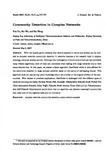
A. Signaling Process. For a network with n nodes, every node is assumed to be a system which can send, receive, and record signals. One node can only affect its neighbors which will affect their neighbors too in the same way. Finally, each node will affect the whole network. In general, one node will affect its community first and then the whole network via its community. So we can safely conclude that the nodes in the same community will affect the whole network in a similar way. At the beginning, we select a node as source and let it has one unit of signal and the other nodes have no signal. Then let the source node send signal to all of its neighbors and itself. After the first step the node and all its neighbors have a signal. In the second step, all the nodes which have signal will send it to their neighbors and themselves. Every node will record the amount of signals it received and then it will send the same quantity of signals in the next time step. In this way, the process will be repeated constantly on the network. After T time steps, we can get a nd vector that records each node’s signal quantity which represents the effect of the source node. The signaling process is sketched out in Fig.1 by simple network with 5 nodes. Choosing every node as the source node respectively, we can get n such vectors. The purpose that we let each node sends signal or signals to itself is to take account of the historical effects. This has been proved to be helpful to distinguish the amounts of signals between the nodes in the community and outside in a relatively short time period. Standardizing the n vectors, then the distance of each pair of vectors will represent the similarity of the corresponding nodes. Using this kind of similarity the communities can be detected. Actually, the above signaling process could be described by a simple but clear mathematical mechanism. Suppose we have a network with n nodes, it can be represented mathematically by an adjacency matrix A with elements Aij if there is an edge from i to j and 0 otherwise. Then the column i of matrix V = (I + A)T will represent the effect of source node i to the whole network in T steps. In order to get the relative effect, we should standardize each column of matrix V. Assume the column i of V is Vi = (vi1 , vi2 ...vin ), v then the Vi can be standardized as Ui = (ui1 , ui2 ...uin ), here uij = Pnijvij . Then to partition j the network which has n nodes is equivalent to cluster n vectors U1 , U2 , · · · , Un in Euclidian space. B. Fuzzy C-mean clustering. It is well known that there are many clustering methods and algorithms for the vectors in Euclidian space. In this paper, we choose the inexpensive fuzzy C-mean clustering algorithm (FCM)[31] to detect communities for the vectors given by signaling process. FCM is described as following. 1. Set C as the number of communities to partition.

4

Figure 1: Sketch of signaling process.(a)We set a signal on node 1 and other nodes have no signal initially. (b)In the first step node 1 sends one signal to all its neighbors which are nodes 2, 3, 4 and 5 and itself. Then all nodes have 1 signal. (c)Next, each of them will send one signal to their neighbors and themselves respectively at the same time. After the second step, node 1 has 5 signals, both node 2 and 3 have 4 signals and node 4 and 5 have 3 signals. Vector [5, 4, 4, 3, 3] represents the effect of the node 1 to the whole network in 2 steps. (d)Then every nodes send the same amount of signals as they received in the last step to their neighbors and themselves. 2. Randomly choose C vectors for the C communities as their barycenters. 3. Randomly choose a vector. The vector will belong to the community when the distance between the vector and the barycenter of the community is minimum among all the barycenter of communities. 4. Re-compute the communities’ barycenters which have added a vector or deleted a vector. 5. Repeat step 3 to step 4 until all the barycenters cannot be modified. We know that there are many definitions of distance. In our algorithm we choose the normal definition–Euclidian distance to measure the similarity between vectors of nodes. C. F Statistic. At the first step of fuzzy C-mean clustering algorithm, we must set an extra parameter C which presents how many clusters we will partition. Here we use F statistic[31] to estimate the proper C. Now let we have a glance at F statistic. Suppose U = {u1 , u2 , · · · , un } is the set of vectors of all nodes and uj = (xj1 , xj2 , · · · , xjn ), here xjk is the kth character quantity of uj . Suppose C is the number of communities and ni is the number of nodes of ith community. Pni iWe name all the nodes’ vectors of the ith community as uj (k) k = 1, 2 · · · , n be the mean characters of ith commuui1 , ui2 , · · · , uini . Let x¯ik = n1i j=1 i i i i nity, u ¯ = (¯ x1 , x ¯2 , · · · , x ¯n ) be the ithP community’s barycenter and u¯ = (¯ x1 , x ¯2 , · · · , x ¯n )be all the nodes’ barycenter, here x ¯k = n1 nj=1 xjk (k = 1, 2, · · · , n). Then F statistic is defined as i 2 P F =

c ni k¯ u −¯ uk i=1 c−1 Pc Pni kuij −¯ui k2 i=1 j=1 n−c

5

,

(1)

250

=4 =5 =6 =7 =8

200

F

150 100 50 0 0

2

4

6

8

C

10

12

14

16

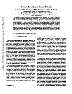
Figure 2: F statistic as the function of number of clusters C. Plot shows the changes of F statistic when T = 3 and hkinter i changes from 4 to 8. It shows that when hkinter i is smaller than 8, F statistic can identify the right number of communities. When the community structure is clearer, the maximal value of F statistic is very distinct. pPm where k u¯i − u ¯ k= xik − x ¯k )2 is the distance between u ¯i and u ¯, and k uij − u ¯i k is the k=1 (¯ i i distance between uj node of ith and the barycenter u¯ . The numerator of F signifies the distance of inter-communities and the denominator the distance of intra-communities. So the F is bigger when the difference distance of inter-communities is bigger and the difference intra-communities is smaller. We can image that when F achieve the maximum we can get the best partition. We use binary ad hoc networks which contains 128 nodes and 4 groups and proceed the signalling process as above to test the F statistic. The results show that F statistic is very efficacious. On the weighted ad hoc networks, the results are similar with binary ones. When the community structure is clearer the maximal value of F statistic is more distinct. The detailed results are shown in Fig.2.

2.2

Some Related Problems

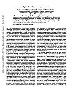
A. The Most Optimal T . Parameter T is an important factor for the results of community identification. We can image that the length T must be sufficiently long to gather enough information about the topology of the network and it should not be too long to faint the information we have gathered. In order to let majority of nodes can affect the whole network and do not to faint the information about the topology of the network, we guess that it may be optimal when T is near to the average shortest path of network. In order to demonstrate our guess, some numerical experiments are done on binary networks which contains 128 nodes and 4 groups as above. The results are shown Fig.3. The accuracy of the algorithm reach optimum when T is 3 or 4. Of course, we only do some numerical experiments, it is 6

accuracy

1.0

0.8

0.6

=4 =5 =6 =7 =8

0.4

0.2 0

2

4

6

8

10

12

14

16

18

20

22

T Figure 3: Let the number of communities be 4 always. The plot shows the changes of accuracy when T changes form 1 to 10 on binary ad hoc networks. From the plots we can see T ≈ 3 is the proper length. And here 3 is near the average shortest paths of each artificial networks. hard to say the result satisfies all the networks. The random walks method[14] has also the same problem. How to find the most optimal T ? We think it is still an open problem. B. Time Complexity analysis. The time complexity of computing F statistic is O(n2 ). For a definite C which is the number of communities, the time complexity for Fuzzy C-mean clustering is O(Cn2 ). Time complexity of the process of signal diffusion is O(T n3 ) when we use the multiplication of matrix to simulate the process. But if we simulate the process in a network directly, the corresponding time complexity is O(T (k + 1)n2 ), where, k is the average degree of node in a network. C. Generalization to weighted networks. It is easy to generalize our algorithm to weighted network. Suppose we have a weighted network with n nodes, it can be represented mathematically by an adjacency matrix W with elements Wij . Wij denotes the connection strength of node i and j (In some weighted network Wij dose not denote the strength of connection, we should transform the weight before the algorithm), then V = (I + W)T . The rest of the algorithm is same with the algorithm on binary ad hoc network. D. Relations with other methods. There two main differences between our method and random walks method and circuit approach method. First, we use the signal diffusion process to transfer the topology to geometrical structure. The mathematical form is (I+A)T . The distance of each pair of column vectors of the matrix is the intimacy of the corresponding pair of nodes. The random walk method gets the intimacy of each pair of nodes by random walks. The mathematical form is (diag( d11 d12 · · · d1n )A)T where, di denote the degree of node i, diag means the diagonal matrix. Take account of the effect of node degree, it also use the Euclidian distance to define the intimacy. The circuit approach method gets the intimacy of each pair of nodes by Kirchhoff’s law. Adding pressure on the proper two nodes, by Kirchhoff’s law, we can get the pressure of each node. More close of the pressure 7

of two nodes are, more intimate the two nodes are. Suppose add pressure on nodes 1 and 2, then p1 = 1, p2 = 0, where pi denotes the pressure of node i. The mathematical ′ ˜ −1 C, where form of Kirchhoff’s law is B = (Adiag( d11 d12 · · · d1n )), (p3 , p4 , · · · , pn ) = (I − B) ˜ denotes the matrix B with deleting the first and the second columns and rows, C = B ′ , Ad41 , · · · , Adn1 ) . Second, as to the method of clustering, we use the F statistic and ( Ad31 3 4 n classical FCM method to partition the vectors. When the F statistic achieve its maximum, we get the best partition. The random walks method and the circuit approach method are all need the help of other indexes to get the best partitions. One is modularity Q, the other is tolerance. So we could say that F statistic and FCM method are all based on the geometrical structure of the vector space, but the other two methods need the help of extra parameters. Because the random walks method and the circuit approach method both need some extra parameters which are very important to the results, so in this paper we will not compare our results with that of these two algorithms in different networks. Instead, we will compare the accuracy and precision with other famous algorithms which do not require any extra parameters.

3

Results and Comparison with other Algorithms

In order to investigate our algorithm, the accuracy and precision of our algorithm will be compared with Potts algorithm(Potts)[16], Girvan-Newman algorithm(GN)[25] and extremal optimal algorithm(EO)[13]. All these algorithms can be generalized to weighted networks[30]. Here we abbreviate GN weighted version as WGN and EO as WEO. The accuracy and precision are defined in [30]. Accuracy means the consistence when the community structure from algorithm is compared with the presumed communities, and precision is the consistence among the community structures from different runs of an algorithm on the same network. The algorithm’s accuracy and precision are calculated by S function[30] in this paper. In the following numerical investigations on ad hoc networks, we first get 20 realizations of artificial community networks under the same conditions. Then we run each algorithm to find communities in each network 10 times. Based on these results, using the similarity function S, comparing each pair of these 10 community structures and averaging over the 20 networks (average of totally C210 × 20 = 900 results) we could get the precision of the algorithm. Comparing each divided groups with the presumed structures, we can get the accuracy of the algorithm by averaging these 10 × 20 = 200 results.

3.1

Results on ad hoc networks

A. Binary ad hoc networks. In order to compare our algorithm with others we first test it on computer-generated random graphs with a well-known predetermined community structure[25]. Each graph has N = 128 nodes divided into 4 communities of 32 nodes each. Edges between two nodes are introduced with different probabilities depending on whether the two nodes belong to the same group or not: every node has hkintra i links on average to its fellows in the same community, and hkinter i links to the outer-world, keeping hkintra i + hkinter i = 16. Fig.4 shows the results. The precision of our algorithm is better than EO and almost the same as Potts and GN. While the accuracy of our algorithm is better than GN and almost the same as EO and Potts. 8

1.0

0.8

0.8

0.6

accuracy

precision

1.0

EO GN

0.4

Potts Signal

0.2

0.6

EO GN

0.4

Potts Signal

0.2

0.0

0.0

0

(a)

1

2

3

4



3

4



Figure 4: Algorithm performance as applied to ad hoc networks with n = 128 and four communities of 32 nodes each. Total average degree is fixed to 16. We can see that the precision of our algorithm is better than EO and Potts and equal GN and the accuracy is better than GN and almost the same as EO and Potts. B. Weighted ad hoc networks. In weighted networks, we use similarity link weight to describe the closeness of relations between nodes. Under the basic construction of ad hoc network described above, the intragroup link weight is assigned as wintra , while the intergroup link weight is assigned as winter . Similarly with hkintra i + hkinter i = 16, we require the link weight on intra and inter links follow the constraint: wintra + winter = 2, where wintra ( winter ) is the average of all intragroup (intergroup) link weights. Here for simplicity, we assign the same weight winter = w to all intergroup links, and assign the same weight wintra = 2 − w to all intragroup links. From Fig.5, we can find that the precision of our algorithm is better than WEO and Potts and equal to WGN, the accuracy of our algorithm is better than WGN but almost equals WEO and Potts. Even for the case with hkinter i < hkintra i but hwinter i > hwintra i, or with uniform distribution of link weights, we can get similar conclusions. C. Complete weighted networks. An extreme idealized example is the complete network. In complete networks, we use uniform distribution of link weights. Weights are taken randomly from the interval [hwintra i−0.25, hwintra i+0.25] and [hwinter i−0.25, hwinter i+0.25] respectively, for intragroup connections and intergroup connections. The precision of our algorithm is better than WEO and Potts and equal to WGN when hwinter i ≪ hwintra i, but its accuracy almost declines to zero when hwinter i is greater than 0.9. Fig.6 shows the results in detail.

3.2

Empirical Results on Some Real Networks

A. Zachary’s karate club. Zachary karate club network[28] has bee considered as a simple sample for community detecting methodologies[10, 19, 21, 9, 23, 25]. This network was constructed with the data collected observing 34 members of a karate club over a period of 2 years and considering friendship between members. We let T = 3 and get the best partition which perfectly corresponds to the actual division of the club Fig.7 9

1.0

0.8

0.8

0.6

accuracy

precision

1.0

WEO WGN

0.4

Potts Signal

0.2

0.6 WEO WGN 0.4

Potts Signal

0.2

0.0

0.0

0.0

0.2

0.4

w

(a)

0.6

0.8

1.0

0.0

0.2

w

(b)

inter

0.4

0.6

0.8

1.0

inter

1.0

1.0

0.8

0.8

accuracy

precision

Figure 5: The influence of weight on community structure when hkintra i = hkinter i = 8, where winter changes from 0.05 to 1. We can see the precision of our algorithm is better than WEO and Potts and equal to WGN and the accuracy of our algorithm is better than WGN but almost equals WEO and Potts.

0.6 WEO GN

0.4

Potts Signal

0.6

GN 0.4

0.2

0.0

0.0

0.4

(a)

0.6



0.6



Figure 6: Precision and accuracy of our algorithm and WGN, Potts, WEO algorithms in complete networks with presumed communities. When hwinter i ≫ hwintra i, the precision of our algorithm is better than WEO and Potts and equal to GN and the accuracy of our algorithm is better than GN always but sharply declines to near 0.2 when hwinter i is greater than 0.9.

10

Figure 7: Our algorithm detects 2 communities form Zachary karate club, which perfectly corresponds the actual division. B. College football network. The algorithm is also applied to College football network which was provided by Mark Newman. The network is a representation of the schedule of Division I games for the 2000 season: vertices in the network represent teams and edges represent regular-season games between the two teams they connect. What makes this network interesting is that it incorporates a known community structure. The teams are divided into 12 conferences. Games are more frequent between members of the same conference than between members of different conferences. The average shortest path length of the football network is 2.5, so we let the signaling time T = 3. When the F statistic achieve the maximum we get the best partition. We also use the accuracy index of detecting community algorithm [30] to measure the effect of our algorithm and find that it identifies the conference structure with a high degree of success. We detect 15 communities when F reach it’s maximum (Fig.8) among which 2 communities just have 2 and 3 teams respectively and five communities were detected absolutely. The average accuracy is 0.78 which is little better than any of others (Tab.3.2).

4

Conclusion

The investigation of community structures in complex networks is an important issue in many domains and disciplines. This problem is relevant to social tasks, biological inquiries, or technological problems. In this paper, we have introduced a method to detect communities based on the signaling process on networks. In a complex networks with n nodes, every node is viewed as a system which can be inspired. Each node sends its neighbors and itself signals and record the number of signals it receives at every time step. For each node of the network, we give it an initial unit quantity signal and other nodes have the signal of zero. Then after the inspiration of T steps on the network, the signal distribution of the nodes denoted by an n-dimensional vector can be

11

120

Value of F statistic

100

80

60

40

20 0

5

10 15 20 Number of community

25

Figure 8: Plot shows the change of the F statistic with the number of communities when T = 2. F statistic achieve its maximum when the number of communities is 15, among which 2 communities just have 2 and 3 teams respectively

Table 1. The accuracy of each detected community compared with the counterpart of real world community Conference name Atlantic Coast Big East Big10 Big12 Conference USA IA Independents Mid American Mountain West Pac10 SEC Sunbelt Western Athletic Average accuracy

FCM accuracy 0.4444 0.8000 1 1 0.9000 0.2500 0.7692 1 1 1 0.4444 0.7273 0.7779

GN accuracy 1 0.8889 1 0.9231 0.9000 0 0.8667 0 0.5556 0.7500 0.4444 0.7273 0.6713

12

EO accuracy 1 0.8000 1 1 0.9000 0 0.9286 0.5714 1 0.7059 0 0.7273 0.7194

Potts accuracy 1 0.8000 1 1 0.9000 0 0.8667 0.5714 1 0.7500 0 0.7273 0.7179

viewed as the influence of the source node to the whole network. The amount of signals be sent is equal to its present-owning signals. In complex networks, we can generally consider that the node always influence its community first then through the community influence the whole network. So naturally, compared with the nodes of other communities, nodes in the same community have similar influence toward the whole network. So through the signaling process, the network partition problem is transformed into the vectors clustering problem in Euclidian space. The clustering can be work out by Fuzzy C-means clustering method(FCM) with the help of F statistic. Moreover, our algorithm can also be generalized to weighted networks when we think the weighted connections can magnify or dwindle the signals linearly. Thus the method presented here can detect the optimal community structures in binary and weighted networks without any extra parameters. To solve the partition problem of complex networks, precision and accuracy of an algorithm are two standards for us to choose the method. So we make a comparison between our algorithm and other relatively mature ones such as EO, Potts and GN algorithms both in binary and weighted networks. Results for both ad hoc and real networks have proved that our algorithm is effective. One problem of our algorithm is that we haven’t given a clear range of the most optimal steps T of inspiring. Actually, some other algorithms such as the random walks method[14] exist also the similar problem. So we think it is an open problem and we will do some deep research on it in the future.

Acknowledgement The authors thank Professor M.E.J. Newman very much for providing College Football network data. This work is partially supported by 985 Projet and NSFC under the grant No.70771011, No.70431002, and No.60534080.

References [1] R. Albert, A.-L. Barabasi, Rev. Mod. Phys. 74, 47 (2002). [2] M. E. J. Newman, SIAM Rev. 45, 167-256 (2003). [3] S. Boccaletti, V.Latora, Y. Moreno, M. Chavez, and D.-U. Hwang, Physics Report. 424, 175-308 (2006). [4] R. Albert, H. Jeong, A.-L. Barabasi, Nature. 401,130 (1999). [5] S.Redner, Eur.Phys. J. B 4, 131 (1998). [6] M. E. J. Newman, Proc. Natl. Acad. Sci, U. S. A. 98,404 (2001). [7] H. Jeong, B. Tombor, R. Albert, Z.N.Oltvai and A.-L.Barabasi, Nature 407,651 (2000). [8] M. E. J. Newman, Proc. Natl. Acad. Sci. U. S. A 103, 8577-8582 (2006). [9] M. Girvan and M. E. J. Newman, Proc. Natl. Acad. Sci. U. S. A 99, 7821-7826 (2004). [10] M. E. G Newman, Phys. Rev. E 69, 066133 (2004). 13

[11] L. Danon, J. Duch, A. Arenas, and A. Diaz-Guilera, J. Stat. Mech. P09008 (2005). [12] S. Lehmann and L. K. Hansen, arxiv.org/abs/physics/0701348 (2007). [13] J. Duch and A. Arenas, Phys. Rev. E 72, 027104 (2005). [14] M. Latapy and P. Pons, Computing communities in large networks using random walks, in Proceedings of the 20th International Symposium on Computer and Information Sciences, ISCIS’05, LNCS 3733, 284-293 (2005). [15] F. Radicchi, C.o Castellano, F. Cecconi, V. Loreto, and D. Parisi, Proc. Natl. Acad. Sci. U.S.A 101, 2658 (2004). [16] J. Reichardt and S. Bornholdt, Phys. Rev. Lett. 93, 218701 (2004). [17] F. Wu and B. A. Huberman, The Eur. Phys. J. B 38,331-338 (2004). [18] A. Clauset, Phys. Rev. E 72, 026132 (2005). [19] J. P. Bagrow and E. M. Bollt, Phys. Rev. E 72, 046108 (2005). [20] S. Muff, F. Rao and A. Caflisch, Phys. Rev. E 72, 056107 (2005). [21] M. E. J. Newman and E. A. Leicht, Proc. Natl. Acad. Sci. USA 104, 9564-9569 (2007). [22] C. P. Massen and J. P. K. Doye, Phys. Rev. E 71, 046101 (2005). [23] L. Donetti and M. A. Munoz, J. Stat. Mech. P10012 (2004). [24] A. Capocci, V. D. P. Servedio, G. Caldarelli, and F. Colaiori, Physica A 352, 669 (2005). [25] M. E. J. Newman, M. Girvan, Phys. Rev. E 69, 026113 (2004). [26] U. Brandes, D. Delling, M. Gaertler, R. Gorke, M. Hoefer, Z. Nikoloski, and D. Wagner, arXiv:physics/0608255, (2006). [27] S. Fortunato and M. Barthelemy, Natl. Acad. Sci. U. S. A. 104, 36 (2007). [28] W. Zachary, Journal of Anthropol Research, 33, 452 (1977). [29] M. E. J. Newman, Phys. Rev. E 74, 036104 (2006). [30] Y. Fan, M. Li, P. Zhang, J. Wu, Z. Di, Physica A 377 (2007). [31] A. Li, Fuzzy mathematics and application. Metallurgical Industry Press. Beijing, (2005). (Chinese book.ISBN-7-5024-3818-1). [32] Image courtesy Mark Newman’s site at http://www.personal.umich.edu/mejn/networks/

14