Compact Layout of Layered Trees. Kim Marriott. Peter Sbarski. Clayton School of IT, Monash University, Australia. {marriott,sbarski}@mail.csse.monash.edu.au.
Compact Layout of Layered Trees Kim Marriott
Peter Sbarski
Clayton School of IT, Monash University, Australia. {marriott,sbarski}@mail.csse.monash.edu.au
Abstract The standard layered drawing convention for trees in which the vertical placement of a node is given by its level in the tree and each node is centered between its children can lead to drawings which are quite wide. We present two new drawing conventions which reduce the layout width to be less than some maximum width while still maintaining the essential layered drawing convention. These conventions relax the requirement that a parent must be exactly placed midway between its children, and instead make this a preference which can be violated if this is required for the layout to fit into the required width. Both drawing conventions give rise to a simple kind of quadratic programming problem. We give an iterative gradient projection algorithm for solving this kind of problem, and also a linear time heuristic algorithm. Our algorithms are practical: a tree with three thousand nodes can be laid out in less than a hundred milliseconds with either algorithm. 1
Introduction
Trees, i.e. connected acyclic graphs, occur in a wide variety of applications, including computer data structures, parse trees, hierarchical database models, phylogenetic trees, hierarchically organised file systems (for example, directories and files), decision trees, organization charts, family trees and biological classifications. Given the practical importance of trees it is not surprising that there has been considerable research into tree layout. The standard layered drawing convention of trees stipulates (Br¨ uggermannKlein & Wood 1989, Kennedy 1996) that: 1. the y-coordinate of each node corresponds to its level, 2. nodes on the same level are separated by a minimum gap, 3. edges do not cross each other, 4. each node is centered directly over its children, 5. the drawing is symmetrical with respect to reflection, 6. the trees are drawn compactly. Wetherell and Shannon (Wetherell & Shannon 1979) proposed a linear time algorithm for layered drawing of binary trees, and this was improved by c Copyright 2007, Australian Computer Society, Inc. This paper appeared at Thirtieth Australasian Computer Science Conference (ACSC2007), Ballarat, Australia. Conferences in Research and Practice in Information Technology, Vol. 62. Gillian Dobbie, Ed. Reproduction for academic, not-for profit purposes permitted provided this text is included.
Reingold and Tilford (Reingold & Tilford 1981). Walker (Walker 1990) extended the Reingold-Tilford algorithm to handle n-ary trees, while Buchheim, J¨ unger and Leipert (Buchheim, J¨ unger & Leipert 2002) gave an improved version of Walker’s algorithm with linear time. The Reingold-Tilford algorithm and the subsequent extensions are the standard methods for drawing rooted ordered trees. However, a disadvantage of these algorithms is that the resulting drawings can be be quite uncompact as the real-world example in Figure 1 shows. In part for this reason, a number of other drawing conventions for trees have been suggested (di Battista, Eades, Tamassia & Tollis 1999). These include radial drawings in which the layers are mapped to concentric circles and hv-drawings in which the edges are either drawn horizontally to the right, or vertically to the bottom. The disadvantage of these other drawing conventions is that the structure and hierarchical nature of the tree is less clear, and the layout looks “unnatural”. We present two new drawing conventions which reduce the layout width to fit in some maximum drawing width while still maintaining the essential layered drawing convention. Both conventions relax the requirement that a parent must be exactly placed at the midway between its children, and instead make this a preference which can be relaxed if this is required for the layout to fit into some maximum width. The drawing conventions give rise to a simple kind of quadratic programming problem in which a quadratic objective must be minimized subject to minimum separation between nodes on each level, and the layout fitting in the maximum width. We give a gradient projection algorithm for solving this kind of problem, and also a linear time heuristic algorithm. Our techniques have application to most realworld visualisation of trees since a significant disadvantage of the standard layered drawing convention is that even for moderate sized trees the drawing becomes quite large and cannot easily be viewed on a computer monitor or printed on a reasonable number of pages. Thus there is a need to find layouts which are more compact and which better untilise the space in a page or on a screen. Figures 2, 3 and 4 show examples of the layout produced by our algorithms for the example from Figure 1. In the next section we review the standard algorithms for layout of layered trees. In Section 3 we present the new drawing conventions, Section 4 contains the algorithms for finding a layout satisfying the conventions, and Section 5 gives an empirical evaluation of their performance, while Section 6 concludes. 2
Background
The Reingold-Tilford algorithm (Reingold & Tilford 1981) uses a divide-and-conquer strategy to find a lay-
Figure 1: Example tree detailing the relationship between Indo-European languages drawn with the Walker Algorithm. out. A single node is placed at 0, and a non-leaf node i is placed by a recursively laying out its sub-trees and then squashing the sub-trees as close as possible together and then placing i midway between the leftmost and rightmost child. Clever use of data structures allows this to be done in linear time. Reingold-Tilford’s algorithm can be modified to handle n-ary trees by traversing the children of a node left to right, placing and shifting the corresponding subtrees one after another. However, this approach may violate the aesthetic goal that the tree must be symmetric with respect to reflection since some branches can end up being clustered closely together as they are placed as close as possible to the left rather than being evenly spaced apart. Walker (Walker 1990) gave a modification of Reingold-Tilford’s algorithm for n-ary tree layout which overcomes this problem. The contours of a node’s sub-trees are traversed, and if there is an overlap, the right subtree is shifted by the minimum amount to the right. Any smaller subtrees situated between the overlapping left and right subtree are uniformly spaced between the two outer sub-trees. This guarantees that the symmetry is preserved. Unfortunately, the algorithm given by Walker has quadratic worst case complexity. Buchheim, J¨ unger and Leipert (Buchheim et al. 2002) improved Walker’s algorithm to have linear time. One nice property of Reingold-Tilford’s and Walker’s approach is that the drawing of a sub-tree does not depend on its context, and so isomorphic subtrees will have the same layout, and that drawings are symmetric with respect to reflection. However, because of this it will not always produce a layout of minimum width, as minimising the over all width may require that some sub-trees are drawn non-compactly. The problem is that minimizing the total width may mean that isomorphic subtrees need to be laid out differently in different parts of the tree as their global context is important. If we do wish to minimize the total width while still placing a parent midway between its children then this can be modelled as a linear programming problem and solved in polynomial time (Supowit & Reingold 1983). However, in practice, the requirement that the parent is exactly midway between its children means that the minimal width layout is only very rarely narrower than that found using ReingoldTilford’s and Walker’s approach. Therefore, in the next section we investigate drawing conventions in which the requirement to place each parent exactly midway between its children is relaxed. As we shall see this allows narrower layout.
3
Drawing Conventions that Relax Centering of Parents
Requiring that parents are midway between their children means that the drawing cannot be as narrow as possible. In this section we give two new drawing conventions for layered trees in which we must find the best layout for the tree that is no wider than some fixed width W . W might be set by the user interactively to try and better fit the layout within a display or print region. Of course, we require that W is greater than the cumulative width of the nodes on each level, since otherwise there is no drawing in which the nodes do not overlap. We assume there are n nodes, 1, ..., n where node 1 is the root of the tree, and 1, ..., m levels with the root on level 1. We let wi give the width of node i, and rt(i) be the index of the node to the immediate right of i on the same level and let gapi give the minimum gap between i and the node to its immediate right. For each level j, lm(j) and rm(j) respectively give the index of the leftmost and rightmost node on that level. We assume that nodes are numbered consecutively on each level. We let xi be the horizontal position of node i. We let par(i) be the index of the parent of i, and lc(i) and rc(i) the index of the leftmost and rightmost child of i (they are the same if i has one child). We use the convention that if the node referred to by indexing function does not exist then the indexing function returns 0: For instance, par(1) returns 0 as the root of the tree has no parent. The first drawing convention is based on making trees compact by minimizing edge lengths. This has the affect of placing nodes at the average of their parent and children’s positions subject to the non-overlap and minimum width constraints. Drawing Convention: Minimizing distance between parents and their children (Min-Dist) Minimize n X (xpar(i) − xi )2 i=2
subject to: for all i ∈ 2, ..., n • xi + w2i + gapi ≤ xrt(i) − and for all j ∈ 1, ..., m, w • 0 ≤ xlm(j) − lm(j) 2 w • xrm(j) + rm(j) ≤ W. 2
wrt(i) 2 ,
if rt(i) 6= 0
This is similar to the objective used in Gansner et al. (Gansner, Koutsofios, North & Vo 1993) to determine the placement of nodes on each layer in a Directed Acyclic Graphs (DAGs) drawn using the Layered drawing convention. Given a horizontal ordering
(a) Min-Dist: W = Wmax
(b) Min-Dist: W = Wmid
(c) Min-Dist: W = Wmin
Figure 2: Example tree from Figure 1 drawn with the Min-Dist drawing convention for different maximum widths W using the gradient projection algorithm. of the nodes on each layer, their algorithm determines the x-coordinates by minimizing edge lengths between nodes. The main difference is that they model this as a linear problem and so minimize n X
|xpar(i) − xi |
i=2
rather than
n X
and parent’s horizontal position, since this minimizes the total horizontal extent of the edges. If placing a parent exactly between its leftmost and rightmost child is regarded as important we can extend the Min-Dist drawing convention by adding another term to the objective function to achieve this:
(xpar(i) − xi )2 .
i=2
As pointed out in (Marriott, Moulder, Hope & Twardy 2005), using a linear objective may lead to unnecessary asymmetry as parents are not necessarily centred with respect to their children since the objective function uses absolute value. Thus, if the root of the tree has two children, it can be placed at any point between these without changing the penalty. Therefore, we prefer to use a quadratic objective function since in the above example this will prefer to place the root midway between its children. However, in general the Min-Dist drawing convention will not place nodes midway between their children but rather at the average of their children
Drawing Convention: Placing parents midway between their children (Par-Midway) Minimize � � n X X xlc(i) + xrc(i) 2 2 (xpar(i) −xi ) +α× xi − 2 1≤i≤n s.t. i=2 rc(i)6=0
subject to: for all i ∈ 2, ..., n • xi + w2i + gapi ≤ xrt(i) − and for all j ∈ 1, ..., m, w • 0 ≤ xlm(j) − lm(j) 2 wrm(j) • xrm(j) + 2 ≤ W .
wrt(i) 2 ,
if rt(i) 6= 0
The scaling coefficient α specifies the relative importance of the two components of the objective. If α is equal to 0, then Par-Midway is identical to the Min-Dist drawing convention, but as α increases in
(a) Par-Midway: W = Wmax , α = 1.0
(b) Par-Midway: W = Wmid , α = 1.0
(c) Par-Midway: W = Wmin , α = 1.0
Figure 3: Example tree from Figure 1 drawn with the Par-Midway drawing convention for different maximum widths W and a small value of α using the gradient projection algorithm. value the resulting layout will tend to place parents midway between their children. It is also worth pointing out that if W is wider than the width of the layout obtained with Walker, then the layout obtained with Par-Midway for large α will be very similar to that obtained by the Walker algorithm. Of course, the main feature of interest is that W can be decreased down to the minimum width for the tree, and the two drawing conventions will “squish” the layout into that width. Figures 2, 3 and 4 show examples of the layout produced by our algorithms for the example from Figure 1 and illustrate the effect of α and W on the layout. We give the layout for three widths: Wmax , the width of the layout using the Walker algorithm; Wmid , the width of the layout of the narrowest possible layout; and Wmid , the average of Wmax and Wmin . We can see that the Min-Dist drawing convention always gives quite compact, narrow layout. 4
Layout Algorithms
In this section we investigate how to find layouts which satisfy the Par-Midway and Min-Dist drawing conventions. Both require minimising a quadratic ob-
jective function of form min xT Ax x
subject to some separation constraints between nodes on the same level where a separation constraint c is of form u + a ≤ v where u, v are variables and a is the minimum gap between them or an upper or lower bound on a variable v of form c ≤ v or v ≤ c. For the Min-Dist drawing convention we have that A is AM D where for each node i, D • AM = deg(i) (where the degree, deg(i), of i is i,i the number of children of i plus the number of parents) and D MD • AM i,par(i) = Apar(i),i = −1
and all other entries in AM D are zero. For the Par-Midway drawing convention we have that A is AP M = AM D + α ×
n X i=1
where for each node i,
Ci
(d) Par-Midway: W = Wmax , α = 1.0E7
(e) Par-Midway: W = Wmid , α = 1.0E7
(f) Par-Midway: W = Wmin , α = 1.0E7
Figure 4: Example tree from Figure 1 drawn with the Par-Midway drawing convention for different maximum widths W for a very large α using the gradient projection algorithm. • if i has no children, C i = 0, • if i has one child c, non-zero entries are i i Ci,i = Cc,c = 1, i i Ci,c = Ci,c = −1
• if i has leftmost and rightmost children l and r, the non-zero entries are i Ci,i = 1, i i Cl,l = Cr,r = 1/4, i i i i Ci,l = Cl,i = Ci,r = Cr,i = −1/2, i i Cl,r = Cr,l = 1/4.
For both drawing conventions the matrix A is symmetric and positive semi-definite. Since separation constraints are linear this means that both conventions require solving a convex quadratic program. 4.1
Iterative Gradient Projection Methods
We now give an iterative gradient-projection algorithm (see Bertsekas (Bertsekas 1999)) for finding a layout for the above kind of problem. It is based on
the gradient projection algorithm given in (Dwyer, Koren & Marriott 2006) but specialized to the particular case of trees. The algorithm, gp layout, is shown in Fig. 5. This works by taking an initial layout, such as that obtained with the Walker algorithm, and then iteratively improving the placement of nodes. At each iteration, the direction of steepest descent, −g, is computed where g is the gradient ∇xT Ax = 2Ax (actually 12 g is computed, but multiplying the descent direction by a constant has no affect). Then the step size s along −g from x that minimizes the objective function is determined and x is set to this new position. Since the new value of x may violate the separation constraints this is corrected by calling project, which returns the closest point x ¯ to x which satisfies the separation constraints, i.e. it projects x on to the feasible region. Finally, a vector d from the initial position x ˆ to x ¯ is computed and a decrease in the objective when moving in this direction is ensured by computing a second stepsize α which minimizes the objective in this interval. While the algorithm given in Figure 5 describes a fairly standard gradient-projection approach, the procedure project is specific to our particular quadratic program. The main difficulty in implementing gradient-projection methods is the need to efficiently
procedure gp layout(A,W ) x ← initial soln() repeat g ← Ax T g s ← ggT Ag x ˆ←x x←x ˆ − sg x ¯ ←project(x, W ) d←x ¯−x ˆ T d α ← min(− dgT Ad , 1) x←x ˆ + αd until kˆ x − xk sufficiently small return x procedure project(x, W ) for j ← 1 to m do g ← [gapi | i ∈ lm(j), ..., rm(j) − 1] d ← [xi | i ∈ lm(j), ..., rm(j)] xlm(j) , ..., xrm(j) ← level project(d, g, W ) end for return x
procedure bottom up narrow(W) x ← walker() for j ← m to 1 do g ← [gapi | i ∈ lm(j), ..., rm(j) − 1] d ← [des(i) | i ∈ lm(j), ..., rm(j)] xlm(j) , ..., xrm(j) ← level project(d, g, W ) end for return x Figure 7: Linear time bottom-up algorithm to layout a tree with n nodes on m levels s.t. the layout is no wider than W and nodes have a minimum separation.
It follows from standard results on gradient projection and the fact that this is a convex optimisation problem that Theorem 1 gp layout converges to a solution that minimizes xT Ax subject to the node separation and maximum width constraints.
Figure 5: Gradient projection algorithm to layout a tree with n nodes on m levels s.t. the layout is no wider than W , nodes have a minimum separation and the position x for the nodes minimizes xT Ax where A is a symmetric positive-semidefinite matrix.
As we shall investigate in the next section, the algorithm is reasonably fast. The matrix A has only O(n) non-zero entries. This means that as long as a sparse representation is used for A, each iteration takes only linear time since the projection step takes only linear time.
project on to the feasible region. That is, we must solve the quadratic problem
4.2
min y
n X
2
(yi − di )
i=1
subject to the same constraints on the variables y as the original problem. Fortunately, the procedure optimal layout given in (Marriott et al. 2005) can be used to project on to the feasible region. It solves the quadratic problem m X wi × (yi − di )2 min y
i=1
subject to a separation constraint of form yi + gi ≤ yi+1 for each i = 1, . . . , m − 1 where gi is the minimum separation between yi and yi+1 , di is the desired position for yi and wi the importance of placing yi at di . The algorithm works by merging variables into larger and larger blocks of variables where a block is a sequence of variables with the minimum gap between each pair. The variables are processed left to right. When variable yi is processed it is placed in a new block b at its desired location di . If the preceding block overlaps b it is merged with b and the desired position of the block is set to the weighted mean of the desired locations of variables in the block. This is repeated until b does not overlap the preceding block. The algorithm has linear complexity. We can use optimal layout to compute the projection for the nodes in a single layer: the only trick is that we add a dummy node at the beginning of the layer and one at the end whose desired values are 0 and W respectively, and whose weight is much higher than that of the other nodes. The two dummy nodes force the other nodes to fit in the desired width for the layout. The procedure level project does this. By combining the projection for each layer, we have the overall projection. Since optimal layout has linear time complexity, the overall projection has linear time complexity.
Bottom-up Algorithm
We have also investigated a one pass bottom-up approach to find a layout satisfying the width restriction. The algorithm is given in Fig. 7. The idea is quite simple. We first determine a layout using Walker’s algorithm. Now we process the layers from the bottom up. For each layer j, we compute the desired position di of each node i in the layer using the function des(i) where if i has children, des(i) is their midpoint (xlc(i) + xrc(i) )/2, otherwise des(i) is the node’s current position xi . The new position, xi , for each node i is computed by using level project to project the desired values on to the closest solution satisfying the minimum width and node separation constraints for that level, effectively squishing them into the width W . Figure 6 shows the layout for various values of W for the examples from Figure 1. It is instructive to compare them with the layouts shown in Figures 2, 3 and 4 obtained using the gradient projection algorithm to find a layout satisfying the Par-Midway drawing convention for α = ∞, since the procedure bottom up narrow can be viewed as a heuristic for finding a layout satisfying this convention. As these examples show, it is not guaranteed to find the optimal solution, but, it will always find a solution satisfying the width and separation constraints, and it does this in linear time assuming the linear time version of Walker’s algorithm is used. 5
Evaluation
To evaluate the efficiency of our algorithms we laid out 10 random trees, with 100 to 3000 nodes. Times can be seen in Table 5. All experiments were run on a 1.83 GHz Intel Centrino with 1GB of RAM. The algorithms were implemented using Microsoft Visual C# Compiler version 8.00.50727.42 for Microsoft .NET Framework version 2.0.50727 under the Windows XP Service Pack 2 operating system. We used the original Walker algorithm
(a) W = Wmax
(b) W = Wmid
(c) W = Wmin
Figure 6: Example tree from Figure 1 drawn for different maximum widths W using the Bottom-up Layout Algorithm. rather than the linear version: as the results show performance of the original algorithm is effectively linear and extremely fast. We used our implementation of the Walker algorithm to compute the initial solution for both the bottom-up and the gradient projection algorithms. We did not include the time taken to compute this initial solution: this is simply the time for running Walker’s algorithm. The tolerance for terminating the gradient projection algorithm was set to 0.002 of the width. The speed of both the gradient projection algorithm and the bottom-up algorithm is very satisfying: even very large trees can be laid out in less than 200 milliseconds and the speed is comparable with that of Walker’s algorithm, the standard layered tree layout algorithm. The main reason for the fast performance of the gradient projection algorithm is that the number of iterations is quite small since the algorithm quickly converges to the optimal layout. 6
Conclusion
The standard layered drawing convention for trees can lead to wide layouts because each parent must be placed exactly midway between its children. We
have introduced two new drawing conventions for layered trees: Min-Dist in which the horizontal distance between parent’s and children is minimised, and ParMidway in which we minimize the horizontal distance between parent’s and their children but also try and minimise the distance between a parent and the midpoint of its children. Thus both drawing conventions relax the requirement that a parent must be exactly placed at the center of its children, and instead effectively make this a preference which can be relaxed if this allows the tree to fit in a drawing of the desired width. We have given an iterative gradient projection based algorithm for computing tree layouts using these two new drawing conventions. Experimental evaluation shows that the algorithm is fast enough for practical applications: a tree with three thousand nodes can be laid out in a few hundred milliseconds, which is only a few times slower than Walker’s algorithm. We have also given a linear-time bottomup algorithm for narrowing a layout produced by the Walker algorithm. This is somewhat faster, with similar speed to Walker’s algorithm, and takes less than 100 milliseconds to layout a tree with over three thousand nodes. The layout quality is also quite good and similar to that of the gradient projection algorithm.
Nodes
Levels
Walker
32 49 52 84 220 365 673 1102 2101 3278
9 9 7 16 16 28 22 201 31 101
18 18 20 21 21 22 24 30 33 36
Min-Dist Wmax Wmin 16 (4) 17 (5) 18 (4) 20 (3) 18 (2) 25 (19) 19 (2) 21 (22) 43 (19) 69 (28) 17 (2) 25 (5) 29 (3) 35 (4) 145 (38) 160 (40) 66 (3) 79 (3) 80 (3) 92 (3)
Par-Midway (α = 1.0) Wmax Wmin 15 (3) 15 (3) 14 (3) 16 (3) 16 (3) 17 (3) 17 (3) 21 (24) 39 (16) 70 (29) 17 (2) 29 (6) 20 (3) 27 (4) 147 (38) 157 (39) 63 (3) 65 (4) 83 (3) 86 (3)
Bottom-up Wmax Wmin 4 4 4 4 4 4 5 4 6 5 7 7 11 11 14 14 26 21 34 31
Table 1: Performance figures for 10 random trees. All timings are given in milliseconds. Figures in brackets specify the number of iterations. The gradient projection algorithm was used to compute the layout for the Min-Dist and Par-Midway drawing conventions. References Bertsekas, D. P. (1999), Nonlinear Programming, 2nd edn, Athena Scientific. Br¨ uggermann-Klein, A. & Wood, D. (1989), ‘Drawing trees nicely with TeX’, Electronic Publishing 2(2), 101–115. Buchheim, C., J¨ unger, M. & Leipert, S. (2002), Improving Walker’s algorithm to run in linear time., in ‘Graph Drawing’, pp. 344–353. di Battista, G., Eades, P., Tamassia, R. & Tollis, I. (1999), Graph drawing: algorithms for the visualisation of graphs, Prentice Hall. Dwyer, T., Koren, Y. & Marriott, K. (2006), IPSepCoLa: An incremental procedure for separation constraint layout of graphs, in ‘Proc. IEEE Symp. on Information Visualisation (Infovis’06)’. Gansner, E. R., Koutsofios, E., North, S. C. & Vo, K.-P. (1993), ‘A technique for drawing directed graphs’, IEEE Transactions on Software Engineering 19(3), 214–230. Kennedy, A. J. (1996), ‘Drawing trees’, Functional Programming 6(3), 527–534. Marriott, K., Moulder, P., Hope, L. & Twardy, C. (2005), Layout of Bayesian networks, in ‘Australasian Computer Science Conference’, Vol. 38. Reingold, E. M. & Tilford, J. S. (1981), ‘Tidier drawings of trees’, IEEE Transactions on Software Engineering 7(2), 223–228. Supowit, K. & Reingold, E. (1983), ‘The complexity of drawing trees nicely’, Acta Informatica 18. Walker, J. Q. (1990), ‘A node-positioning algorithm for general trees’, Software Practice and Experience 20(7), 685–705. Wetherell, C. & Shannon, A. (1979), ‘Tidy drawings of trees’, IEEE Transactions on Software Engineering 5(5), 514–520.