Comparing Classification Approaches for Mapping ...

Comparing Classification Approaches for Mapping Cut-leaved Teasel in Highway Environments Cuizhen Wang, Diego J. Bentivegna, Reid J. Smeda, and Randy E. Swanigan

Abstract Cut-leaved teasel is an invasive weed thriving in roadside environments and needs to be detected for implementation of management programs. This study tested several commonly applied classifiers to map teasel with an aerial hyperspectral image along the Interstate Highway 70 in central Missouri. A teasel/non-teasel mask was first built to exclude dominant land-covers that had distinct spectral differences from teasel. The spectral angle mapping (SAM) had the best results of delineating teasel from herbaceous background with its user’s and producer’s accuracies of 80 to 90 percent. Large commission errors of teasel were observed in the probability-based maximum likelihood classifier (MLC) and spectral information divergence (SID) methods. Compared with a regular land-use/land-cover classification in an unsupervised/supervised hybrid method, the post-masking SAM had much easier process of training data collection and achieved similar accuracies. It could be an optimal approach for mapping teasel and other weeds in highway environments.

Introduction Cut-leaved teasel (Dipsacus laciniatus L.), hereafter referred as teasel, is an invasive, biennial weed that often infests roadside environments (Solecki, 1993). Following emergence, it grows as a rosette in the first year and bolts and flowers in the second year (Werner, 1975). A flowering plant is able to produce 33,500 seeds distributed within one meter around the parent plant (Bentivegna, 2008). As plants die after seed production, newly developed rosettes fill in the open areas. As a result, teasel patches observed in natural environments are often composed of flowering plants up to 2 to 3 meters and understory rosettes, producing a dense canopy with a leaf area index up to 3 (Bentivegna, 2008).

Cuizhen Wang is with the Department of Geography, University of Missouri, 8 Stewart Hall, Columbia, MO 65211 ([email protected]). Diego J. Bentivegna is with the CERZOS, Camino de la Carrindanga Km 7, Bahía Blanca B8000FWB, Buenos Aires, Argentina. Reid J. Smeda is with the Division of Plant Sciences, University of Missouri, 204 Waters Hall, Columbia, MO 65211. Randy E. Swanigan is with the Missouri Department of Transportation, Jefferson City, MO 65102. PHOTOGRAMMETRIC ENGINEERING & REMOTE SENSING

Teasel patches could reduce traffic visibility on highways. The aggressive colonization of teasel patches also eliminates desirable grass species along roadsides (Solecki, 1993). In the United States, teasel has been declared as noxious weed in four states including Missouri (USDA, 2008). Responsible for management of vegetation along roadsides, the Missouri Department of Transportation (MoDOT) often chooses site-specific or selective herbicide applications to optimize herbicide use efficiency. The conventional in-situ surveys to locate teasel invasion, however, are time consuming and are impractical for statewide road systems. Field visits are also extremely hazardous to highway workers. Remote sensing techniques provide an efficient way for large-area mapping of weed infection. Multispectral imagery has been widely applied to detect invasive plants in various open areas (Carson et al., 1995; Lass et al., 1996; Medlin et al., 2000; Shaw, 2005). However, few applications have been attempted in roadside environments. Due to low maintenance along roadside right-of-ways, teasel often establishes into small, heterogeneous patches mixed with native species. As herbaceous vegetation, teasel has similar spectral properties as grasses such as tall fescue (Festuca arundinacea) that are commonly observed along roadsides in Missouri. Therefore, it is often difficult to discriminate teasel patches from dominant grasses with typical aerial photos. For this reason, hyperspectral imagery is necessary to identify the subtle spectral differences among vegetation types in mixed environments (Ustin et al., 2004, Wang et al., 2008). Another aspect that is often considered in weed detection is the unique phenological features of the weed in certain growth stages (Lawrence et al., 2006; Nagendra, 2001; Underwood et al., 2003). For example, Lass et al. (1996) reported that yellow starthistle (Centaurea solstitialis) could be best mapped with remote sensing imagery acquired in the flowering stage, when yellow flowers exhibited distinctively different spectra from other vegetation. Teasel grows in compact patches and white flowers could be observed in mid-late July in Missouri. Imagery acquired in this period may provide optimal information for mapping teasel along highways. With multispectral imagery, various classification algorithms have been developed in vegetation studies.

Photogrammetric Engineering & Remote Sensing Vol. 76, No. 5, May 2010, pp. 567–575. 0099-1112/10/7605–0567/$3.00/0 © 2010 American Society for Photogrammetry and Remote Sensing May 2010

567

Among these algorithms the most commonly applied one is the maximum likelihood classifier (MLC), a supervised classifier that examines the statistical properties of training data and assigns a pixel to the class with the highest probability (Jensen, 2004). When hyperspectral imagery became available, new classifiers were developed to take advantage of the nearly continuous spectra. These classifiers treat each pixel as an n-dimensional vector to compare the spectral similarity between image spectra and reference spectra, the so-called endmemebers. The spectral angle mapping (SAM) is the most widely applied classifier in hyperspectral remote sensing. It calculates the angles between each pixel vector and endmember, and then assigns the pixel to the class with the smallest angle (Kruse et al., 1993). As a result, it is a deterministic measure of the ndimensional Euclidean distance between the pixel and endmember. Contrarily, the newly developed spectral information divergence (SID) performs a stochastic measure that examines statistical properties of endmembers (Du et al., 2004). Different from the MLC, the SID does not consider the second-order statistical moments (e.g., variance, covariance) of endmembers. Rather, it defines a probability vector for each pixel by calculating the probability distribution of digital numbers in the spectrum, and then compares the divergence between the pixel and endmember. The pixel is assigned to the class with least divergence. Therefore, the SID follows a combined decision rule of the MLC (probabilities) and the SAM (continuous vectors). The application of these classifiers in roadside environments is uncertain. Due to the heterogeneous distribution of land-covers, weed patches are often small and narrowly distributed along highways. Although modern aerial images could reach pixel size of one meter or less, mixed pixels are inevitable in these patches. Moreover, the MLC assumes that each class has an equal probability of occurring in the landscape (Jensen, 2004). It is not valid in this study because the invasive teasel is not dominant in highway environments. For the SAM and the SID, it is often difficult to find representative endmembers in these patches. Calculation of angular distances or divergences in these classifiers may be largely negated by mixed pixels and large spectral variation when teasel grows in a composition of flowering plants and rosettes. In mixed environments the SAM could result in much lower accuracy than the conventional MLC algorithm (Shafri et al., 2007). This study tested the feasibility of teasel mapping in roadside environments with these three classifiers. A stepwise decision tree was first built to mask out trees, healthy grasses, water, and impervious surfaces that had distinct spectral differences from teasel. The MLC, SAM, and SID classifiers were then applied to map teasel/non-teasel using an aerial hyperspectral image acquired along the Interstate Highway 70 (I-70) in central Missouri. Spectral signatures of teasel were collected from ground reference data and error matrices were built to compare the accuracies of these classifiers. The optimal classifier was suggested to MoDOT for practical weed mapping in highway environments.

Materials and Methods Study Area and Data Set The study area was along I-70 in Cooper County, Missouri. A 2.5 km section close to Exit 89 was selected because the area was heavily infested with teasel. White flowers in teasel patches could be observed in mid-late July in Missouri. Soil was a silt loam distributed along steep slopes with scattered rocks. Tall fescue was the most common grass 568

May 2010

species growing in the study area. Undesirable herbaceous species, such as sericia lespedeza (Lespedeza cuneata), johnsongrass (Sorghum halepense L.), and common milkweed (Asclepias syriaca L.) could also be observed. Tall fescue-dominated pastures/hayfields and trees were common land-covers off the highway. A hyperspectral image was acquired on 25 July 2006 by the Center for Advance Land Management Information Technologies (CALMIT), University of Nebraska, using the Airborne Imaging Spectroradiometer of Applications (AISA) (Plate 1A). The AISA image contained 63 bands in the spectral range of 401 to 981 nm (visible-near infrared (NIR)) at 1 m spatial resolution. The spectral resolution was approximately 10 nm. The image delivered by CALMIT had been geometrically corrected, radiometrically calibrated, and atmospherically corrected using the Fast Lineof-sight Atmospheric Analysis of Spectral Hypercubes (FLAASH) algorithm (ENVI, 2006). Several field surveys were conducted in 2006. Ground control points were collected with a differential GPS unit that could reach an accuracy of one meter. It was found that the root-meansquare error (RMSE) of these points in the AISA image was less than one pixel. With a digital camera mounted on a low-altitude light airplane, a set of true-color aerial photos along I-70 in the study area were collected on 19 July 2007. At a flight height of 1,500 meters, the photos reached a fine pixel size of 0.5 m. Without built-in positioning and moving compensation capability in the system, it was extremely difficult to correct the geometrical distortions of these photos. In this study, these photos were primarily used to visually compare with the AISA image to locate ground reference data. One photo taken at Exit 89 showed the largest teasel patch in the study area (Plate 1B). An example ground picture of teasel patch is displayed in Plate 1C. Twenty rectangular plots along I-70 in the study area were selected during field surveys for studies of herbicide treatment (Bentivegna, 2008). Except for one plot that was out of the image extent, locations of these plots are marked in Plate 1A. Teasel covered more than 50 percent of these plots. Constrained by topography along I-70, these plots ranged from 5 to 13 meters wide and 10 to 34 meters long with an average area of 190 meter2. Teasel in each plot was vigorously green during the AISA image acquisition and could be identified by visualizing the image and the matching 0.5 m aerial photos. As an example of demonstration, teasel patches in the largest two plots at Exit 89 are outlined in Plate 1B. It has to be noted that the aerial photos were taken one year after the AISA image. A majority of flowering teasel plants were killed with herbicide treatment by MoDOT in early-July 2007, although some rosette remained green when aerial photos were taken. These two teasel patches served as training data to build teasel signatures for classification of the AISA image. Teasels in other plots were treated as ground validation data. Theoretical Basis of Classifiers For an image with n bands, any pixel could be defined as a vector x ⫽ (x1, x2. . . . .xn)T, in which the components are the reflectance values of band 1 to n. A classifier compares image vector with reference vectors under stochastic (MLC, SID) or deterministic (SAM) rules. Maximum Likelihood Classifier (MLC) The MLC decision rule is based upon the probability that a pixel belongs to each class. For class i, training pixels are extracted from the image and the mean vector mi, as well as inter-band covariance matrix Vi, are calculated. Under the assumption of normal distribution of training data in each PHOTOGRAMMETRIC ENGINEERING & REMOTE SENSING

(c)

(b)

(a)

Plate 1. (a) The AISA image (wavelengths of 472.35 nm, 544.67 nm, and 638.19 nm are displayed) in the study area, and (b) a 0.5 m aerial photo of a large teasel patch at Exit 89. A teasel picture taken on the ground (July 2006) is displayed in (c). Ground teasel polygons are marked in red in (a), and the two largest teasel polygons are outlined in (b).

class, the probability that a pixel vector x belongs to class i could be calculated as (Jensen, 2004): MLC(x)i ⫽

1 (2p) ƒ Vi ƒ n 2

1 2

exp c ⫺

1 (x ⫺ mi )T Vi⫺1( x ⫺ m i ) d . 2

(1)

The pixel is assigned to the class in which it has the highest probability of occurring. Spectral Angle Mapping (SAM) The SAM is an n-dimensional distance measure between a pixel and each reference endmember. For class i, the endmember vector (ei) is composed of mean reflectance value of all training pixels in each band. The angle between x and ei is calculated as (Kruse et al., 2003): SAM (x)i ⫽ cos⫺1 a

8x,ei9 ‘x‘

#

‘ ei ‘

b

n

⫽ cos ⫺1≥

a xj ei,j

j⫽1

1 a a xj2 b 2 j⫽1 n

1 2 2 a a ei,j b j⫽1 n

¥

(2)

where xj and ei,j are the reflectance values of x and ei in band j, respectively. The pixel is assigned to the class with the smallest angle. PHOTOGRAMMETRIC ENGINEERING & REMOTE SENSING

Spectral Information Divergence (SID) The SID is endmember-based as the SAM while it follows a stochastic rule as the MLC. For a pixel vector x, the probability of a reflectance value (␳) that occurs at band b can be calculated as (Chang, 2000): pb ⫽

rb n

.

(3)

a rl

l⫽1

The cross entropy, or directed divergence, between the probability vectors of the pixel and each endmember is then calculated. Please refer to Chang (2000) for a detailed calculation. The pixel is assigned to the class with the smallest divergence. Image Preprocessing: A Stepwise Teasel/Non-teasel Mask As a first attempt to map teasel in the study area, Bentivegna (2008) performed a hybrid unsupervised/supervised classification using the AISA image. Without a priori knowledge, the research first grouped all pixels in the image into 300 clusters using the ISODATA (Iterative SelfOrganizing Data Analysis Techniques) algorithm. These 300 clusters were further grouped into 20 classes based upon the clusters’ spectral variability, the analyzer’s familiarity with the study area, and visualization of the 0.5 m aerial photos. As shown in Figure 1, the 20 classes May 2010

569

Figure 1. The 20 training signatures after the ISODATA clustering. These training spectra were applied in a regular 20-class LULC mapping with the MLC and SAM algorithms (Modified from Bentivegna, 2008).

are: (1) teasel, (2) water, (3) bare surface, (4) tree, and (10) grass. Bare surfaces are composed of paved roads and ground surfaces without vegetation cover. Trees include broadleaves, conifers, and shrubs that are commonly observed along I-70. As the dominant land-covers, grasses are represented by 10 classes because of the heterogeneous composition of species and greenness in the highway environments. In Figure 1, the spectrum of teasel is clearly different from water, paved bare surfaces and trees, but could be confused with some grasses. Water has low reflectance and impervious surfaces have high reflectance in the visibleNIR region. Trees and very healthy dense grasses are characterized with high reflection in near infrared and high absorption in red bands. For these vigorous vegetation types, there is an apparent water absorption trough at 933 nm, a feature that is able to be identified in narrow bandwidths of the AISA image. This absorption trough cannot be observed in teasel and sparse, less healthy grasses. The normalized difference vegetation index (NDVI) could differentiate most non-vegetation and healthy vegetation. However, at 1 m pixel size, the AISA image reveals large areas of shaded tree canopies and grasses. By normalizing the spectral responses in red-NIR region, the NDVI was designed to reduce the effects of soil background (Tucker, 1979). It was also not sensitive to shadows in forest stands (Huemmrich, 1996; Wang et al., 2005). In the AISA image, the shaded healthy vegetation reaches similar NDVI values as teasel and non-healthy grasses. Similarly, the water absorption trough at 933 nm is not clear in shaded areas. When examining the spectral profiles of shaded vegetation, we noticed that its reflectance in blue-green region was much lower than teasel. Using the same formula as NDVI, we 570

May 2010

defined a normalized difference shadow index (NDSI) to extract shaded areas in this study: NDVI ⫽

r761 ⫺ r676 r761 ⫹ r676 (4)

NDSI ⫽

r554 ⫺ r436 r554 ⫹ r436

where r436,r554, r675, and r761 are reflectance values at wavelengths of 436 nm, 554 nm, 676 nm, and 761 nm, respectively. The NDVI and NDSI of different classes are compared in Figure 2. It is obvious that healthy tree canopies in the woodland, as well as some green herbaceous patches along I-70, reaches the highest NDVI (Figure 2a). Water and paved driveways have the lowest NDVI values. The shaded vegetation (e.g., at the edges of woodland) shows dramatic differences in NDVI and NDSI images. Its NDVI values tend to be similar as those of pasture grasses while its NDSI values are much lower (dark tones in Figure 2b). As described in the flow chart in Figure 3, a stepwise mask is built using criteria of the reflectance at 933 nm, NDVI and NDSI. A combined rule of “NDVI ⬎0.5 & r933nm ⫽ local minimum” is used to detect trees and healthy grasses. The results are not optimal when these rules are applied independently. With “NDVI ⬎0.5” itself, large areas of grasses in pastures/hayfields could not be masked, which increases the possibility of teasel overestimation. With “r933nm⫽local minimum” itself, some teasel pixels are included, resulting in teasel underestimation. The “NDVI ⬍0.2” detects nonvegetation such as water and bright bare surfaces. The “NDSI ⬍0.3” detects shaded vegetation and some non-vegetation PHOTOGRAMMETRIC ENGINEERING & REMOTE SENSING

(a)

(b)

Figure 2. Example images of (a) NDVI, and (b) NDSI in a subset area in north of I-70. A water body, pasture field, and a piece of woodland are covered in the subset.

Results

Figure 3. Framework of a stepwise masking process to extract dominant land-covers of trees, healthy grasses, water, and impervious surfaces in the AISA image. The r933 nm represents the reflectance at wavelength 933 nm.

that cannot be selected in previous steps. After trees, healthy grasses, water and impervious surfaces are masked out of the AISA image, the remaining pixels are primarily teasel and non-healthy grasses. These two classes are hereafter referred to as teasel and non-teasel. The postmasked AISA image is processed with the MLC, SAM, and SID algorithms to perform a simplified teasel/non-teasel mapping in the study area. PHOTOGRAMMETRIC ENGINEERING & REMOTE SENSING

Regular LULC Classification: Teasel Mapping in a Past Study (Bentivegna, 2008) With the 20 training signatures extracted after the ISODATA clustering (Figure 1), Bentivegna (2008) performed the MLC classification using the AISA image. The resultant 20 classes were re-grouped into five land-covers: teasel, water, bare surface, grass, and tree. Using the 20 signatures as endmembers, the SAM classification was also performed. The maximum angle threshold of 10° was used as it provided optimal results when the threshold was tested in a range of 5° to 30°. The pixel was defined as “unclassified” if the spectral angle between this pixel and each endmember was larger than this threshold. Similarly, the resultant 20 classes were regrouped into the five landcovers mentioned above. The study found that only teasel patches at relatively large sizes along I-70 could be detected using both MLC and SAM algorithms. Water, bare surfaces, and trees were easily classified, but strong confusion between teasel and grasses was observed in both classifiers. Large areas of grasses (even those in pastures/hayfields) were misclassified as teasel in the SAM class map. Bentivegna (2008) also performed accuracy assessment of the two class maps. Adopting a stratified random sampling method (Congalton, 1991), a total of 250 points (50 for each class) were randomly selected all over the study area. Each point represented the major class in an area of 5 ⫻ 5 pixels centered at this point. The reference classes of these points were identified using field observations and visualization of the 0.5 m aerial photos. In the error matrices of the two classifiers (Table 1), teasel and grasses always had the lowest accuracies compared to water, bare surfaces, and trees. When all classes were considered, the overall accuracy of the MLC (92.4 percent) was much higher than that of the SAM (76.8 percent). However, the overall accuracy was not representative in teasel mapping because teasel was not the May 2010

571

TABLE 1.

ERROR MATRICES OF THE MLC AND SAM CLASS MAPS IN A REGULAR LAND-USE/LAND-COVER CLASSIFICATION IN (FROM BENTIVEGNA (2008)). DIAGONAL VALUES ARE IN BOLD TO EMPHASIZE THE CORRECT ALLOCATIONS

THE

STUDY AREA

Ground Reference Teasel

Grasses

Bare surfaces

Trees

Teasel Grasses Bare surfaces Trees MLC class map Water Column_total Producer’s accuracy Overall classification accuracy: 92.4% Kappa value: 0.91

41 2 2 1 0 46 89.1%

5 47 2 2 0 56 83.9%

4 1 46 0 0 51 90.2%

0 0 0 47 0 47 100%

Teasel Grasses Bare surfaces Trees SAM class map Water unclassified Column_total Producer’s accuracy Overall classification accuracy: 76.8% Kappa value: 0.71

29 15 1 1 0 0 46 63%

7 43 4 2 0 0 56 76.8%

3 2 40 0 0 6 51 78.4%

0 3 0 42 0 2 47 89.4%

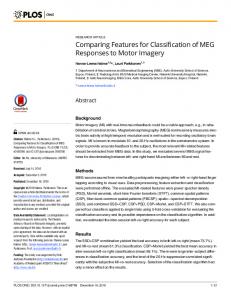
dominant class in the study area. For teasel itself, the user’s and producer’s accuracies in the MLC map were 82 percent and 89.1 percent, respectively. The respective accuracies were only 74 percent and 63 percent in the SAM class map. This indicated that, when all land-covers were considered in a regular LULC classification, the ISODATA/MLC algorithm was better applied for mapping teasel in highway environments. Post-masking Classification: Teasel/Non-teasel Mapping After trees, water, and impervious surfaces were masked out of the AISA image, training data of teasel and non-teasel (mostly non-healthy grasses) were visually selected based on the 0.5 m aerial photos. The training area of teasel contained 247 pixels in the two teasel plots at Exit 89. The training data of non-teasel contained 214 pixels along vegetated roadsides in the north of the teasel plots. Areas farther away from I-70 were not considered in training area selection. All training pixels were used in the MLC classification. The mean spectrum of training pixels of the classes served as endmembers in the SAM and SID approaches. The MLC assigned each pixel in the post-masking AISA image to teasel or non-teasel. There was an obvious overestimation of teasel in the MLC class map (Plate 2). A large number of patches along I-70 were classified as teasel. Large grass fields, such as the ones in the middle of the image (north of I-70) and the lower right of the image (south of I70), were also assigned as teasel. Since there was no “unclassified” category in the MLC algorithm, pixels with low probability values in the training data were also processed. For example, there was a large pond in pastures in the middle of the study area. Its border areas could not be masked out because the shallow, muddy water often had high chlorophyll content from phytoplankton or wetland vegetation, which resulted in high NDVI values. These areas were assigned as teasel in the MLC map. The post-masking SAM and SID algorithms dramatically reduced the overestimation of teasel in the study area. In the SAM map, major teasel patches along I-70 right-of-ways were 572

May 2010

Water

Row_total

User’s accuracy

0 0 0 0 50 50 100%

50 50 50 50 50 Total: 250

82% 94% 92% 94% 100%

0 0 0 0 38 12 50 76%

39 63 45 45 38 20 Total: 250

74.4% 68.3% 88.9% 93.3% 100%

detected (Plate 2). Most grass fields that were misclassified in the MLC map were correctly assigned as non-teasel. The abovementioned pond was identified as “unclassified.” The SID map was similar as the SAM map, but there was a slightly higher overestimation of teasel in pastures/hayfields, although the overestimation was much lower than the MLC map (Plate 2). Accuracy Assessment In the stepwise masking process, the NDVI and NDSI thresholds of non-teasel classes were selected in a way to maximally avoid assigning teasel in the mask. As shown in the class maps in Plate 2, large areas of non-healthy grasses were not masked out because of their spectral similarity with teasel plants. It was also discovered in the past study that the confusion between teasel and other classes (except grasses) was small (Table 1). For the 20 ground-observed teasel plots, we found that none of them were masked out. Therefore, the accuracy of the masking map was acceptable in this study. Due to limited teasel population and small patch sizes along highways, it was not possible to randomly select a large number of ground reference data of teasel for its accuracy assessment. For this reason, a randomized cluster sampling strategy (Congalton, 1988) was applied to extract ground reference data from the selected teasel plots. In each plot, pure teasel polygons were traced by comparing the AISA image with the matching 0.5 m aerial photos. These teasel polygons were mostly in size of 10 to 20 pixels. Although spatial autocorrelation among these teasel pixels were inevitable, it was reported in Congalton (1988) that the effect of spatial dependency of clustered samples in accuracy assessment could be reduced when cluster sizes were small. A total of 372 teasel pixels in 17 plots were extracted as ground validation data. Similarly using photo visualization, seven patches of non-healthy grasses were randomly selected (five along I-70 and two in pastures/hayfields off I-70) in the AISA image. A total of 377 pixels were extracted as ground reference data of non-teasel. PHOTOGRAMMETRIC ENGINEERING & REMOTE SENSING

(a)

(b)

(c)

Plate 2. The teasel/non-teasel class maps with (a) MLC class map, (b) SID class map, and (c) SAM class map algorithms in the study area. The AISA image is displayed in the masked background.

With these ground data, the error matrix approach (Congalton, 1991) was used to assess the accuracies of the MLC, SID, and SAM class maps. In the error matrices of the three teasel/non-teasel maps (Table 2), the MLC had the lowest overall accuracy (61.2 percent) while the SAM reached the highest accuracy (86.8 percent). The obvious overestimation of teasel in the MLC class map in Plate 2 resulted in its high producer’s accuracy (94.6 percent) and low user’s accuracy (56.5 percent). Similarly, the SID class map had high producer’s accuracy of 92.5 percent and low user’s accuracy of 65.9 percent. The SAM class map achieved much better results of teasel mapping with high values in both producer’s (82 percent) and user’s (90.5 percent) accuracies. The accuracies were also evaluated based on the kappa coefficient of agreement derived for each classification. As listed in Table 2, the MLC, SID, and SAM had the Kappa values of 0.22, 0.45, and 0.74, respectively. The Kappa analysis may not be appropriate in comparing the three classifications with the same set of ground data because it assumed indePHOTOGRAMMETRIC ENGINEERING & REMOTE SENSING

pendent samples in different assessments (Foody, 2004). The uncertainties rising from this situation, however, could be small in this study when the kappa values varied largely among the three classifications. With much easier process of training data selection, the post-masking SAM approach in this study reached similar accuracies as the complicated unsupervised/supervised (ISODATA/MLC) hybrid classification in the past study (Table 1). It indicated that, when only teasel and non-teasel classes were considered, the SAM might be better applied for mapping teasel in highway environments.

Discussion Weed detection along roadsides is different from open-area environments because of the distinctive dynamic of landcovers in long, narrow ground surfaces. Spectral properties of the same vegetation type may vary dramatically in different locations, due primarily to the heterogeneity in May 2010

573

TABLE 2.

ERROR MATRICES OF THE MLC, SAM, AND SID CLASS MAPS IN THE POST-MASKING TEASEL/NON-TEASEL MAPPING STUDY; DIAGONAL VALUES ARE IN BOLD TO EMPHASIZE THE CORRECT ALLOCATIONS Teasel

MLC class map

Non-teasel

IN THIS

Row_ total

User’s accuracy

Teasel Non-teasel Column_total Producer’s accuracy

352 20 372 94.6%

271 106 377 54.6%

623 126 Total: 749

56.5% 84.1%


305 67 372 82%

32 345 377 91.5%

337 412 Total: 749

90.5% 83.7%


344 28 372 92.5%

178 199 377 52.8%

522 227 Total: 749

65.9% 87.7%

Overall accuracy: 61.2% Kappa Coefficient: 0.22 SAM class map

Overall accuracy: 86.8% Kappa Coefficient: 0.74 SID class map

Overall accuracy: 72.5% Kappa Coefficient: 0.45

species, density, growth stages, soil fertility, water availability, and other biophysical conditions. Agricultural lands close to the I-70 in Missouri are mostly a mixture of perennial crop fields, whose spectra also vary upon different management activities such as haying and grazing. Regular supervised classification in these environments is highly limited because of the difficulties in collecting representative training data sets. Bentivegna (2008) demonstrated the feasibility of an unsupervised/supervised hybrid classification method to map teasel patches in highway environments. The process is time consuming and subjective when re-grouping ISODATAresulted clusters into representative classes. Uncertainties are introduced with large spectral variation in small teasel populations in the study area. It takes full consideration of all teasel pixels in one image to build a training signature to reach accuracies of 82 to 89.1 percent for teasel. Because of the complexity in processes, this approach could not be easily adopted by end-users such as the MoDOT for statewide application. Many studies have shown that the SAM classifier with hyperspectral imagery can reach much higher accuracies in land-use/land-cover mapping (Kruse et al., 1993; South et al., 2004; Du et al., 2004; Ustin et al., 2004). This classifier, as well as the newly developed SID method, however, did not reach the expected results in highway environments. Compared with the regular multi-class MLC method, these algorithms resulted in higher confusion between teasel and grasses. The low accuracy is primarily attributed to mixed pixels and large spectral variation in small, narrow teasel patches along roadside right-of-ways. Results in this study agree with Shafri et al. (2007) who reported that, for a seven-class tree mapping in mixed forests with hyperspectral imagery, the overall accuracy of the SAM method was less than 50 percent while the MLC reached 85 percent. Specifically in weed detection, the complexity of landcover mapping in highway environments is reduced by applying a mask to exclude the dominant classes that have distinct spectral differences from target weeds. The stepwise teasel/non-teasel mask in this study excludes trees, healthy grasses, water, and impervious surfaces. While only two classes (teasel and non-healthy grasses) are considered in the classification, the process of training data selection is much easier and the requirement of pure endmembers in 574

May 2010

classifiers with hyperspectral imagery is reduced. By simply identifying a small subset of training area for teasel and nonteasel classes in the image, the SAM algorithm reached similar accuracies as the unsupervised/supervised hybrid (ISODATA/MLC) method in a regular multi-class classification. Contrarily, with the same training data of teasel and nonteasel, the MLC algorithm resulted in large commission errors of teasel in the study area. Different accuracies of these classifiers are rooted in their decision rules. The probability-based MLC algorithm in teasel/non-teasel mapping could not reach the expected accuracy. Due to teasel’s large spectral variation in small training areas, its probability distribution of training data is much wider than that of the non-teasel, which results in high overestimation of teasel patches in the study area. The SAM approach compares the n-dimensional spectral similarity between a pixel and endmembers. The inter-class confusion is dramatically reduced when there are only two classes. The in-class spectral variation is also reduced when training data sets are averaged into two endmembers. Therefore, the confusions in the SAM are much lower than the MLC. Following a combined decision rule of the MLC and SAM, the SID algorithm has higher overestimation of teasel than the SAM, although the extent of overestimation was much lower than the MLC. This study indicated that the post-masking SAM algorithm could reach relatively high accuracy in teasel/non-teasel mapping in highway environments. Compared with the complicated training data collection in the ISODATA/MLC method that has to be performed in each image, the SAM is more advantageous in roadside applications because endmembers collected in one image could be applied in adjacent ones. This is extremely useful in highway systems where mapped areas are narrow and long, covering a large number of scenes. Teasel mapping demonstrated in this study provides important inputs for site-specific weed management for agencies like MoDOT. Instead of heavy workflow of field visits, the MoDOT people only need limited training efforts to monitor highway teasel invasion and treatment when proper imagery becomes available. Despite of its great potential, statewide application of hyperspectral remote sensing is highly limited by image availability. Some research has been investigated to select the most weed-sensitive spectral bands to promote the less PHOTOGRAMMETRIC ENGINEERING & REMOTE SENSING

expensive multi-spectral application. The unique water absorption wavelength centered at 933 nm in this study also reveals the possibility of selecting spectral regions in teasel detection. Moreover, plant phenology plays an important role in weed detection. As more and more high-resolution airborne and spaceborne imagery becomes available, the mapping approaches examined in this study could potentially become practical in weed control in highway environments. Further investigation will be conducted to examine the effectiveness of wavelength selection and multi-temporal image analysis in operational teasel mapping along Missouri highways.

Conclusions This study compared the MLC, SAM, and SID classifiers to map invasive cut-leaved teasel in highway environments using an aerial hyperspectral image that covers 63 bands in visible-NIR region. The uniqueness of the research was the small, narrow teasel patches with large spectral variation along roadside right-of-ways. Major findings about roadside teasel mapping included: 1. For a regular multi-class LULC mapping, the unsupervised/supervised (ISODATA/MLC) hybrid approach provided much higher accuracies than other classifiers. However, the training data selection was time-consuming and the classification process was complicated; 2. A stepwise mask was built with combined criteria of NDVI, NDSI and a near-infrared narrowband (centered at 933 nm, at which healthy vegetation has an apparent absorption trough). Large areas of trees, healthy grasses, water, and impervious surfaces were removed to simplify the process of teasel mapping; 3. With much easier process of training data collection, the SAM teasel/non-teasel mapping achieved similar accuracies (80 to 90 percent) as the ISODATA/MLC method. Due to spectral variation of teasel in small and mixed patches, the probabilitybased classifiers such as MLC and SID resulted in large overestimation of teasel. The SAM may be an optimal algorithm for extended teasel mapping in highway environments.

Acknowledgments This study was partially supported by funding from the Missouri Department of Transportation (MoDOT). We would like to thank Dr. Harlan L. Palm at the Division of Plant Sciences, University of Missouri for his assistance in image acquisition and field work. We also highly appreciate the time and efforts of Dr. Rick Perk at CALMIT, University of Nebraska, and Mr. John Harris, a local vender of real-time aerial photos, in collecting aerial images for this study.

References Bentivegna, D.J., 2008. Integrated Management of the Invasive Weed Cut-leaved Teasel (Dipsacus laciniatus L.) along Missouri highways, PhD dissertation, University of Missouri, 132 p. Carson, H.W., L.W. Lass, and R.H. Callihan, 1995. Detection of yellow hawkweed (Hieracium pretense) with high resolution multispectral digital imagery, Weed Technology, 9:477–483. Chang, C.I., 2000. An information-theoretic approach to spectral variability, similarity, and discrimination for hyperspectral image analysis, IEEE Transactions on Information Theory, 46:1927–1932. Congalton, R.G., 1988. Using spatial autocorrelation analysis to explore the errors in maps generated from remotely sensed data, Photogrammetric Engineering & Remote Sensing, 54(5):587–592. PHOTOGRAMMETRIC ENGINEERING & REMOTE SENSING

Congalton, R.G., 1991. A Review of assessing the accuracy of classifications of remotely sensed data, Remote Sensing of Environment, 37:35–46. Du, Y., C.I. Chang, H. Ren, C.C. Chang, and J.O. Jensen, 2004. New hyperspectral discrimination measure for spectral characterization, Optical Engineering, 43:1777–1786. ENVI, 2006. The environment for visualizing images, ENVI Tutorials, Version 4.3. Research System Institute. Foody, G.M., 2004. Thematic map comparison: Evaluating the statistical significance of differences in classification accuracy, Photogrammetric Engineering & Remote Sensing, 70(6):627–633. Huemmrich, K.F., 1996. Effects of shadows on vegetation indices, Proceedings of the International Geoscience and Remote Sensing Symposium, Lincoln, Nebraska, 4:2372–2374. Jensen, J.R., 2004. Introductory Digital Image Processing: A Remote Sensing Perspective, Third Edition, Prentice Hall, Upper Saddle River, New Jersey, 526 p. Kruse, F.A., A.B. Lefkoff, J.B. Boardman, K.B. Heidebrecht, A.T. Shapiro, P.J. Barloon, and A.F.H. Goetz, 1993. The Spectral Image Processing System (SIPS) - Interactive visualization and analysis of imaging spectrometer data, Remote Sensing of Environment, 44:145–163. Lass, L.W., H.W. Carson, and R.H. Calliham, 1996. Detection of yellow starthistle (Centaurea solstitialis) and common St. Johnswort (Hypericum perforatum) with multispectral digital imagery, Weed Technology, 10:466–474. Lawrence, R.L., S.D. Wood, and R.L. Sheley, 2006. Mapping invasive plants using hyperspectral imagery and Breiman Cutler classifications (RandomForest), Remote Sensing of Environment, 100:356–362. Medlin, C.R., D.R. Shaw, P.D. Gerard, and F.E. LaMastus, 2000. Using remote sensing to detect weed infestation in Glycine max, Weed Science, 48:393–398. Nagendra, H., 2001. Using remote sensing to assess biodiversity, International Journal of Remote Sensing, 22:2,377–2,400. Shafri, H.Z.M., A. Suhaili, and S. Mansor, 2007. The performance of maximum likelihood, spectral angle mapper, neural network and decision tree classification in hyperspectral image analysis, Journal of Computer Science, 3:419–423. Shaw, D.R., 2005. Translation of remote sensing data into weed management decisions, Weed Science, 53:264–273. Solecki, M.K., 1993. Cut-leaved and common teasel (Dipsacus laciniatus L. and D. Sylvestris Huds.): Profile of two invasive aliens, Biological Pollution: The Control and Impact of Invasive Exotic Species (B.N. McKnight, editor), Indianapolis: Indiana Academy of Science, pp. 85–92. South, S., J. Qi, and D.P. Lusch, 2004. Optimal classification methods for mapping agricultural tillage practices, Remote Sensing of Environment, 91:90–97. Tucker, J.J., 1979. Red and photographic infrared linear combinations for monitoring vegetation, Remote Sensing of Environment, 8:127–150. Underwood, E., S. Ustin, and D. DiPietro, 2003. Mapping non-native plants using hyperspectral imagery, Remote Sensing of Environment, 86:150–161. USDA, 2008. The PLANTS Database, version 3.5. National Plant Data Center, Baton Rouge, Louisiana, URL: http://plants.usda .gov (last date accessed: 01 February 2010). Ustin, S.L., D.A. Roberts, J.A. Gamon, G.P. Asner, and R.O. Green, 2004. Using imaging spectroscopy to study ecosystem processes and properties, BioScience, 54:523–534. Wang, C., J. Qi, and M. Cochrane, 2005. Assessment of tropical forest degradation with canopy fractional cover from Landsat ETM⫹ and IKONOS imagery, Earth Interactions, 9(22):1–18. Wang, C., B. Zhou, and H.L. Palm, 2008. Detecting invasive sericia lespedeza (Lespedeza cuneata) in mid-Missouri pastureland using hyperspectral imagery, Environmental Management, 41:853–862. Werner, P.A., 1975. The biology of Canadian weeds 12, Dipsacus sylvestris Huds, Canadian Journal Plant Science, 55:783–794. (Received 19 March 2009; accepted 18 June 2009; final version 31 August 2009) May 2010

575