A first interesting analysis compares the performance of GCF and. OGCF to a suboptimal ..... significant difference between the six algorithms in the 30dB case.
COMPARISON BETWEEN DIFFERENT SOUND SOURCE LOCALIZATION TECHNIQUES BASED ON A REAL DATA COLLECTION Alessio Brutti, Maurizio Omologo, Piergiorgio Svaizer Fondazione Bruno Kessler - irst via Sommarive, 18 38100 Trento, Italy Email: {brutti,omologo,svaizer}@fbk.eu ABSTRACT Comparing the different sound source localization techniques, proposed in the literature during the last decade, represents a relevant topic in order to establish advantages and disadvantages of a given approach in a real-time implementation. Traditionally, algorithms for sound source localization rely on an estimation of Time Difference of Arrival (TDOA) at microphone pairs through GCC-PHAT. When several microphone pairs are available the source position can be estimated as the point in space that best fits the set of TDOA measurements by applying Global Coherence Field (GCF), also known as SRP-PHAT, or Oriented Global Coherence Field (OGCF). A first interesting analysis compares the performance of GCF and OGCF to a suboptimal LS search method. In a second step, Adaptive Eigenvalue Decomposition is implemented as an alternative to GCC-PHAT in TDOA estimation. Comparative experiments are conducted on signals acquired by a linear array during WOZ experiments in an interactive-TV scenario. Changes in performance according to different SNR levels are reported. Index Terms— Source localization, microphone arrays, adaptive eigenvalue decomposition, generalized cross correlation. 1. INTRODUCTION During last years, the problem of locating a sound source in space has received a growing interest from the scientific community. Many audio processing applications can obtain substantial benefits from the knowledge of the spatial position of the source which is emitting the signal under process. For this reason many efforts have been devoted to investigating this research area and several alternative approaches have been proposed over the years [1]. Traditionally, algorithms for sound source localization rely on an estimation of Time Difference of Arrival (TDOA) at microphone pairs from which one can derive information about the spatial position of an emitting source. In this paper we present an experimental comparison, conducted on real data collections, of two TDOA estimation methods, namely Generalized Cross-Correlation PHAse Transform (GCCPHAT) and Adaptive Eigenvalue Decomposition (AED), when combined to source localization based on acoustic maps. Experiments are conducted on excerpts of a WOZ data collection acquired in a domestic-like environment during the DICIT project whose focus This work was partially supported by the EC under the STREP Project DICIT (FP6 IST-034624).
is a user-friendly interface that allows interaction with TV and infotainment services1 . The acoustic setup adopted in the recordings consists of a compact microphone array of 15 microphones deployed in front of the speakers. Ground truth positions for each user were available based on an automatic video tracking [2]. In this paper we first recall GCC-PHAT and AED theories and properties. Then, a description of three different acoustic map computations is presented in Section 3. Section 4 reports the results of our comparative analysis while conclusions and future work close this paper in Section 5. 2. COHERENCE MEASURES Given the signals acquired by a couple of microphones, a coherence measure can be defined as a function that indicates the similarity degree between the two signals realigned according to a given time lag. Coherence measures can hence be used to estimate the time delay between two signals. For example, Cross-Correlation is the most straightforward coherence measure. The most common approach adopted in the sound source localization community to compute a coherence measure is the use of GCC-PHAT [3]. Let us consider two digital signals x1 (n) and x2 (n) acquired by a couple of microphones, GCC-PHAT is defined as follows: ff X1 · X2∗ GCC-PHAT(d) = IFFT (1) |X1 ||X2 | where d is a time lag, subject to |d| < τmax , while X1 and X2 are the DFT transforms of x1 and x2 respectively. The inter-microphone distance determines the maximum valid time delay τmax . It has been shown that, in ideal conditions, GCC-PHAT presents a prominent peak in correspondence of the actual TDOA. On the other hand, reverberation introduces spurious peaks which may lead to wrong TDOA estimates [4]. An alternative way to obtain a coherence measure is offered by AED [5, 6] that is able to provide a rough estimation of the impulse responses that describe the wave propagation from one acoustic source to two microphones. Under the assumption that the main peak of each impulse response identifies the direct path between the source and the microphone, the TDOA can be estimated as the time difference between the two main peaks. Let us denote with h1 and 1 Further
details can be found in http://dicit.fbk.eu
This is a technical report on an activity partially supported by the EC under the STREP Project DICIT (FP6 IST-034624). This work was published at HSCMA 2008 and copyright is held by IEEE.
h2 the two impulse responses, in ideal conditions, i.e. without noise, the following equation holds: h2 ∗ x1 (n) = h2 ∗ h1 ∗ s(n) = h1 ∗ x2 (n)
(2)
where s(n) is the signal emitted by the source. If we consider the vectors u = [h1 , −h2 ] and x = [x1 , x2 ], it can be shown that u corresponds to the eigenvector ˘associated ¯ to the null eigenvalue of the covariance matrix Rx = E x · xT : Rx u = 0
(3)
In noisy conditions, equation 3 does not hold strictly any longer but u, and hence the two impulse responses, can be still computed as the eigenvector corresponding to the h i smallest eigenvalue. The estiˆ 1 , −h ˆ 2 is obtained through an adaptive ˆ = h mated eigenvector u algorithm, as for instance a frequency domain adaptive LMS as presented in [7]. If L is the length of the impulse responses to estimate, u is in general initialized in such a way that h2 (L/2) = 1 while ˆ 2 is forced to be a sort of the reminder is equal to 0. In this way h delta impulse, while the position of the peak in ˆ h1 adapts according to the real TDOA (a peak will rise in L/2 when the TDOA is 0). When the above initialization is adopted, the coherence measure can be derived as: ˆ 1 (L/2 + d) AED(d) = h (4) Although comparisons between GCC-PHAT and AED have been already conducted in the literature [8], they are limited to TDOA estimation capabilities and to simulated data collections. In particular, it is worth noting that in [5, 8] AED turned out to be superior with respect to GCC-PHAT under reverberant and noisy conditions. In our case, instead, we focus on the final localization results and real data and compare GCC-PHAT and AED in combination with acoustic maps, which are introduced in the next section. 3. ACOUSTIC MAPS When several microphone pairs are available, as for instance in the cases of a distributed microphone network or a linear microphone array, the source position can be estimated as the point in space that best fits a set of TDOA measurements. A very efficient solution is offered by acoustic maps which are functions, defined over a sampled version of the space of potential solutions, representing the plausibility that a source is present at a given point. Once a representation of the acoustic activity distribution in an enclosure is available in the form of an acoustic map, the position of the source can be derived as the point that maximizes such a map. Global Coherence Field (GCF) [9], also known as SRP-PHAT, is a very efficient and powerful tool to compute acoustic maps. If we assume that M microphone pairs are available and we can compute a coherence measure Ci (·) at each microphone pair i for every physically valid time delay, GCF is defined as follows: GCF (p) =
M −1 1 X Ci (Ti (p)) M i=0
(5)
where Ti (p) denotes the theoretical time lag at microphone pair i when the source is in p (the lag can be approximated by the closest integer delay). GCF proved to be very efficient in a distributed microphone network scenario [10].
Later on, the newly introduced Oriented Global Coherence Field (OGCF) [11] was shown to be able to provide more accurate and reliable estimates of the source position [12]. OGCF estimates also the orientation of the source through a proper weighting of single Ci (·). This information is then exploited to improve the position estimation accuracy. Unfortunately, in a compact array scenario, as the one taken into account in this paper, the localization capabilities of OGCF can not be fully exploited due to lack of angular coverage provided by the sensor setup. A third interesting method for acoustic map computation implements a suboptimal Least Squares (LS) search method. In this case the plausibility function is computed as follows [13]: LS (p) = −
M −1 1 X |Ti (p) − τi |2 M i=0
(6)
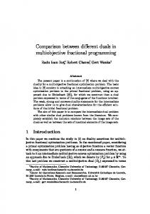
where τi is the time delay that maximizes Ci (·) and corresponds to the TDOA estimation. The minus in equation 6 is introduced to fit the acoustic map definition which requires high scores for points with high plausibility. This method is referred to as suboptimal because it minimizes the LS criterion on a sampled version of the space of source coordinates. From a theoretical point of view LS is weaker than GCF and OGCF since it maintains only the information about the maximum peak at each single microphone pair, while GCF and OGCF use all the information in Ci (·). Anyway it offers a lighter solution from a computational and memory point of view and in some applications it may turn out to be sufficiently accurate. In particular such a solution is very suitable for a compact array setup where users are supposed to be frontal. Conversely, LS is expected to perform worse than GCF and OGCF in a distributed microphone network scenario, with microphones all around the walls of a room. Finally, LS can operate on a continuous domain of time lags since TDOA estimates can be refined, for instance through parabolic interpolation, and there is no need for rounding Ti (p). In a GCF or OGCF approach, instead, interpolation of the whole Ci (·) is very computationally demanding and not reasonable in real time applications. 4. EXPERIMENTAL SETUP AND RESULTS The experimental setup, that is outlined in Figure 1, resembles the application scenario envisioned in the DICIT project: up to four persons are in a room and control an interactive television. The entire sensor setup includes 13 microphones arranged in a harmonic fashion (with an overall distance between the first and the last one of 192 cm) plus two microphones placed 20 cm above the two extremities in order to derive clues for 3D speaker localization. In the following experiments we exploit only a subset composed of 7 sensors with a uniform distance of 32 cm (see Figure 2). The sampling rate is 48kHz and the reverberation time is about 0.65 s. The comparative analysis was conducted on chunks of a WOZ database which was collected for evaluation and development of speech processing technologies under the DICIT project. In our experiments we focused on the very beginning of each session when each speaker is asked to read some phonetically rich sentences while sitting in the positions depicted in Figure 1. Although the data set includes a large amount of signals where users interact freely with the system and move in the room, we restricted our analysis to the first phase mainly to ensure a sufficient reliability of the ground
This is a technical report on an activity partially supported by the EC under the STREP Project DICIT (FP6 IST-034624). This work was published at HSCMA 2008 and copyright is held by IEEE.
linear array
2.1m
3.4m
P4
000 111 111 000 000 111 000 111 000 111
111 000 000 111 000 111 000 111 000 111
P3
P2
111 000 000 111 000 111 000 111 000 111
P1
poorer than GCF and OGCF in noisy conditions, independently of the coherence measure it is combined with. The explanation is related to the fact that in noisy conditions some τi are wrong and directly affect localization performance, while GCF and OGCF can rely also on the information of secondary peaks which is maintained in Ci (·). GCF and OGCF give very similar performance, as it was expected in a compact array scenario, since OGCF potential is only partially utilized. 100
5m
90
80
70 Pcor (%)
Fig. 1. Layout of the experimental setup. 4 positions were investigated at 2.1 m distance from a linear microphone array.
60
50 GCF-GCC OGCF-GCC LS-GCC GCF-AED OGCF-AED LS-AED
40
30 0
Fig. 2. Configuration of the harmonic linear array. The circled sensors form a uniform array of 7 elements.
5
10
15 SNR (dB)
20
25
30
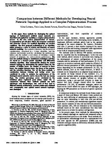
Fig. 3. Localization performance in terms of Pcor for each of the algorithms under investigation when different SNR are applied.
The above analysis is partly confirmed by Figure 4, which reports experimental results in terms of RMSE. It can be observed, however, that under clean conditions AED offers more accurate estimations than GCC-PHAT. This behaviour can be explained with the adaptive nature of AED which takes advantage from the given scenario where sources do not move. As a matter of fact, speech signals are characterized by short pauses, hesitations and portions of signals with energy concentrated in the lower part of the spectrum, which negatively influence the coherence measure evidence. For instance, it has been shown that GCC-PHAT is more reliable when a speaker pronounces a fricative than during a vowel. The adaptive nature of AED, that intrinsically integrates information over time, allows a better bridging of low-coherence segments, which results in an improved overall accuracy. 1200 GCF-GCC OGCF-GCC LS-GCC GCF-AED OGCF-AED LS-AED
1100 1000 900 RMSE (mm)
truth reference coordinates. As a matter of fact, spatial labeling, obtained through automatic video tracking, and manual segmentation are prone to errors which may affect the algorithm comparison. Hence we limited the analysis to more controlled conditions where references are easier to extract and control. Recorded signals include a background of real environmental noise, resulting in an average SNR of 30dB. Three additional SNR levels were then produced by addition of white gaussian noise, which provided average SNRs of 17dB, 7dB and 2dB. Overall, six different localization algorithms are evaluated, which are obtained by combining two coherence measure approaches, i.e. GCC-PHAT and AED, and three acoustic map computation methods, namely GCF, OGCF and LS. We refer to them as: GCF-GCC, OGCF-GCC, LS-GCC, GCF-AED, OGCF-AED and LS-AED. For each of them, acoustic maps are computed on a two dimensional space sampled with 5 cm resolution. Algorithms are evaluated in terms of euclidean distance between reference positions and localization outputs. Due to different time resolutions between algorithms and references, each localization output is associated to a proper reference as described in [10]. Time resolution of the reference positions, which determines the evaluation time resolution, is 0.2 s. A localization error is labeled either as gross, when it is larger than 0.5 m, or as fine otherwise. With “Localization Rate” (Pcor) we measure the reliability of an algorithm as the percentage of fine errors over all the localization estimates. Localization accuracy is measured in terms of “Root Mean Square Error” (RMSE) of all the localization errors (fine and gross). Figure 3 shows performance in terms of Pcor for each algorithm when different SNR levels are applied. SNR equal to 30dB refers to the clean case where no white noise is added and signals are only corrupted by the environmental noise. Notice how there is no significant difference between the six algorithms in the 30dB case while GCC-PHAT performs better than AED as soon as the SNR is lower than about 15dB. It is worth noting also how LS is always
800 700 600 500 400 300 200 0
5
10
15 SNR (dB)
20
25
30
Fig. 4. Localization performance in terms of RMSE for each of the algorithms under investigation when different SNR are applied.
In an effort to verify this interpretation, we consider a post-
This is a technical report on an activity partially supported by the EC under the STREP Project DICIT (FP6 IST-034624). This work was published at HSCMA 2008 and copyright is held by IEEE.
processing on localization estimates based on thresholding of the acoustic map maximum peak. Those estimations which are derived from a low peak, i.e. from not very reliable acoustic maps, are skipped. In order to quantify the consistency of skipped estimates, we introduce a new metric, named “Deletion Rate” (Del), that measure the percentage of speech instants for which an estimation is not available. Post-processing is applied only to the clean case and different thresholds are used, resulting in different Deletion Rates. Figure 5 shows the localization performance of four algorithms in terms of RMSE corresponding to different values of Del. It can be observed how performance of GCC-PHAT equals that of AED already when only few localization estimates are discarded (Del < 5%). It is also worth noting how LS performs slightly better than GCF in the clean case because it can operate without the need of sampling the TDOA domain. GCF-GCC LS-GCC GCF-AED LS-AED
[1] M. Brandstein, D. Ward, Microphone arrays, Springer, 2001. [2] O. Lanz, “Approximate Bayesian Multibody Tracking”, IEEE Transactions on Pattern Analysis and Machine Intelligence,Vol. 28, No. 9, pp. 1436-1449, 2006.
[4] Benoˆıt Champagne, St´ephane Bedard and Alex Stephenne, “Performance of time-delay estimation in the presence of room reverberation” IEEE Transactions on Speech and Audio Processing, vol. 4, pp. 148-152, 1996
260 240 RMSE (mm)
6. REFERENCES
[3] C. Knapp, G. Carter, “The generalized Correlation Method for Estimation of time Delay” IEEE Transactions on Acoustic, Speech and Signal Processing, vol. 4, pp. 320-327, 1976.
300 280
main issue. Evaluation of different localization methods with different acoustic sensor configurations, as for instance distributed microphone networks against a compact microphone arrays, is another research line we are going to investigate next. Finally, this comparative study will be extended to the multiple speaker scenario. In this case a proper acoustic map processing must be applied in order to identifies all the peaks raised by multiple simultaneous speakers [14]
220
[5] J. Benesty, “Adaptive eigenvalue decomposition algorithm for passive acoustic source localization,” Journal of Acoustical Society of America, vol 107, pp 384-391, 2000.
200 180 160 140 0
10
20
30
40
50
Del (%)
Fig. 5. Localization performance in terms of RMSE when a thresholding is applied on localization outputs. The figure takes into account GCF-GCC, LS-GCC, GCF-AED and LS-AED in the 30dB SNR case.
5. CONCLUSIONS AND FUTURE WORK In this paper we proposed a comparative study on the performance of two different approaches for time delay estimation in a sound source localization context. Experiments on a real data collection show that there is no significant difference when the environmental conditions are not very noisy. When the level of noise increases, GCC-PHAT provides better performance than AED. On the other hand the adaptive nature of AED guarantees a less noisy estimation of the position of a static source in the clean case. It is worth remarking that AED is considerably more demanding than GCC-PHAT from a computational complexity point of view, due to the iterative nature of its eigenvector estimation. As a side effect our experiments also prove that under fair SNR conditions LS is as accurate and precise as GCF and OGCF and overcomes them in the clean case. Integration of particle filtering and combination with speaker ID cues are activities currently under investigation in an effort to further enforce localization capabilities of acoustic maps based on the presented algorithms. Future activities will deal with an analysis of these localization algorithms in a moving speaker context where the need for very accurate spatial and temporal references is the
[6] S. Doclo, M. Moonen, “Robust adaptive time delay estimation for speaker localization in noisy and reverberant acoustic environments,” EURASIP Journal on Applied Signal Processing, vol. 2003, pp 1110-1124, 2003. [7] G. Doblinger, “Localization and Tracking of Acoustical Sources,” in Topics in Acoustic Echo and Noise Control, Springer, Berlin - Heidelberg, 2006. [8] J. Chen, J. Benesty, Y. Huang, “Time Delay Estimation in Room Acoustic Environments: An Overview”, EURASIP Journal on Applied Signal Processing, vol. 2006, pp. 1-19, 2006. [9] M. Omologo, P. Svaizer, R. DeMori, Spoken Dialogue with Computers, Chapter 2, Academic Press, 1998. [10] M. Omologo, P. Svaizer, A. Brutti, L, Cristoforetti, “Speaker Localization in CHIL lectures: Evaluation Criteria and Results,” MLMI 2005: Revised and selected papers, pp. 476-487, 2005. [11] A. Brutti, M. Omologo, P. Svaizer, “Oriented Global Coherence Field for the estimation of the head orientation in smart rooms equipped with distributed microphone arrays,” in Proceedings of Interspeech, 2005, pp. 2337-2340 [12] A. Brutti, M. Omologo, P. Svaizer, “Speaker Localization based on Oriented Global Coherence Field”, in Proceedings of Interspeech, 2006, pp. 2606-2609 [13] D. Rabikin et al, “A DSP implementation of Source Location Using Microphone Arrays”, in Proceedings of the 131st Meeting of the Acoustical Society of America, 1996, pp. 88-99 [14] A. Brutti, M. Omologo, P. Svaizer, “Localization of multiple speakers based on a two step acoustic map analysis”, in Proceedings of ICASSP, 2008.
This is a technical report on an activity partially supported by the EC under the STREP Project DICIT (FP6 IST-034624). This work was published at HSCMA 2008 and copyright is held by IEEE.