Proceedings of the 6th Nordic Signal Processing Symposium - NORSIG 2004 June 9 - 11, 2004 Espoo, Finland
Comparison of Continuous- and Discrete-Time Modelling of Polynomial-Based Interpolation Filters Vesa Lehtinen, Djordje Babic, and Markku Renfors Tampere University of Technology Institute of Communications Engineering P.O. Box 553, FIN-33101 Tampere, FINLAND Email: {vesa.lehtinen,markku.renfors}@tut.fi,
[email protected]
ABSTRACT Polynomial-based interpolation filters provide a flexible means for arbitrary and asynchronous sample rate conversion. They can be modelled with a continuous-time piecewise-polynomial impulse response. In sample rate conversion by rational factors, however, only discrete points of the impulse response affect the output signal. This leads to a discrete-time model of the interpolator. In this paper, properties of the continuous- and discrete-time models in optimisation of filters for sample rate conversion are discussed and compared so that the best model can be chosen for each filter design task. Interpolators optimised using the discrete-time model are optimal when a rational conversion factor is fixed. However, interpolators optimised using the continuous-time model can be more robust against changes of the conversion factor, which property is useful in applications that require flexibility.
µ ( k – 1 )T in
( k + 1 )T in
( k + 2 )T in
( k + 3 )T in
Fig. 1. The principle of interpolation filtering. The continuoustime signal represented by a discrete-time sequence is reconstructed at the time instants (k+µ)Tin.
0 0
1. INTRODUCTION Sample rate conversion (SRC) by rational factors is needed in, e.g., digital multimode communication receivers, where the ratios between the sampling rate of the analogue-todigital converter and the symbol/chip rates of different communication standards cannot all be integers in practise. Another typical application is in digital audio systems, where rational SRC is needed in interconnection of devices that conform to different standards. The most straightforward way to realise rational SRC is to perform up- and downsampling by integer factors and anti-image/antialias filtering between them. The structure can be optimised by avoiding multiplications by zero samples and computation of unused output samples. [1, pp. 88–91]. Polynomial-based interpolation filters provide a more flexible approach that is often also more efficient, and most importantly, is feasible also when the SRC factor is a ratio of two large integers or even irrational. For rational SRC, these filters have been optimised using both continuous-time (CT) and discrete-time (DT) models. These models have benefits and drawbacks that have not
1
2 3 4 5 Time in input sample intervals
6
Fig. 2. A typical CT impulse response of a polynomial-based interpolation filter.
been sufficiently analysed before. The purpose of this paper is to give the reader insight to the models and allow the selection of the best model for each filter design task. 2. POLYNOMIAL-BASED INTERPOLATION AND THE FARROW STRUCTURE The principle of interpolation filtering is illustrated in Fig. 1. A continuous-time signal is reconstructed at desired time instants from a sequence of its samples. As parameters, the interpolation filter is given the input sample index k and the fractional interval µ ∈ [0, 1) for each desired output sample. Polynomial-based interpolation filters produce a piecewise-polynomial reconstruction of the signal. A typical CT impulse response of a polynomial-based interpolation filter is shown in Fig. 2. [2] The Farrow structure [3], depicted in Fig. 3, is a convenient and efficient implementation form for polynomial-based variable filters, including interpolators. Its impulse response taps are polynomials in a control variable. In interpolation, the control variable is a function
This work was carried out in the project “Advanced Signal Processing Techniques for Future Wireless Communications Transceivers” supported by the Academy of Finland. The work was also supported by Tampere International School in Information Science and Engineering (TISE) and Nokia Foundation.
©2004 NORSIG 2004
kT in
49
C3(z) z –1
↑K
@F p
H DT ( z )
↓L
@F out
Fig. 5. The discrete-time model for rational decimation.
C0(z)
C2(z)
z –1
C1(z)
@F in
(interpolator): n h DT [ n ] = h CT ⎛ ⎛ --- + µ bias⎞ T ⎞ , ⎝⎝ L ⎠ ⎠
α(µ)
where µbias is a bias used for choosing the sampling phase. The bias has an effect on the magnitude and phase response [8][9]. The DT frequency response is defined as the Fourier transform of the CT impulse response. Calculation of the discrete-time impulse response for different Farrow variants has been discussed in [8]. Notice that the DT model depends on L and µbias. Moreover, in irrational SRC, µ takes an infinite number of different values, hence the DT model does not exist. For purposes of Section 4, we define LT as the target value of L, i.e., the value used when designing the filter. The value of L used in the realisation is denoted by LR.
Fig. 3. The Farrow structure. For the Modified Farrow structure, α(µ)=2µ–1. DT @F in
CT
H CT ( s )
(3.1)
@F out
Fig. 4. The continuous-time model for fractional sample rate conversion. of the fractional interval. A number of modifications have been developed: The Modified Farrow structure improves efficiency by exploiting coefficient symmetry [2]. The transposed Farrow structure [4][5] provides good antialiasing properties for decimation (the original Farrow structure has poor antialiasing performance). Also other variants have been proposed. In this paper, only the Modified and transposed Modified Farrow structure are considered but most of the results apply to other variants as well.
4. COMPARISON OF THE MODELS For comparison, a set of interpolators were optimised for different signal bandwidths, attenuation specifications, and values of LT. Cases with a single continuous stopband and multiple stopbands (comprised of the bands aliasing to the passband) were considered. In each case, the same subfilter lengths and polynomial degrees were used for the CT design and all target conversion ratios of the DT model, with exceptions explained below. For the DT designs, µbiasing [9] was used in order to obtain the best performance. The peak stopband ripple levels of the DT frequency responses of a few example filters are shown in Figs. 6–9 as functions of LR. In the plots, M and N denote the polynomial degree and number of polynomial segments of the filter, respectively. The passband edge fp is normalised so that unity corresponds to half of the sample rate in the subfilters. Only minimax optimisation was considered in the comparison. It can be observed that the peak ripple depends on LR. The reason is that, in the sampler of the CT model, multiple images of a given input frequency alias to the same output frequency. Their phase differences depend only on the filter HCT(s), not on the input phase. The summation of these aliases can be either constructive (deteriorates attenuation) or destructive (improves attenuation) depending on the phase response of the filter. At different values of LR, the aliasing patterns of images of a given input frequency are different, resulting in different peak ripple levels in the DT model. When LR approaches infinity, the DT ripple level approaches that of the CT frequency response, whereas the maximum attenuation loss is suffered at the lowest values of LR. Fig. 10 shows that the value of LR below which significant attenuation loss occurs is almost independent of the polynomial
3. INTERPOLATOR MODELS 3.1 Continuous-time model SRC by any factor can be modelled with the system presented in Fig. 4 [1, pp. 22–29]. The input sample sequence is converted into the equivalent continuous-time train of weighted Dirac impulses, filtered with a CT reconstruction filter and then sampled at the output sample rate. From the frequency-domain point of view, the purpose of the reconstruction filter is to reject images and/ or limit the bandwidth in order to avoid aliasing. A typical CT impulse response is shown in Fig. 2. The CT frequency response is defined as the Fourier transform of the CT impulse response. 3.2 Discrete-time model In interpolation by a rational factor L/K (with K