Comparison of multiple linear regressions and artificial intelligence ...

AJAE 3(2):39-46 (2012)

ISSN:1836-9448

Comparison of multiple linear regressions and artificial intelligence-based modeling techniques for prediction the soil cation exchange capacity of Aridisols and Entisols in a semiarid region Yusef Kianpoor Kalkhajeh1*, Ruhollah Rezaie Arshad1, Hadi Amerikhah1, Moslem Sami2 1 2

Department of Soil Science, Faculty of Agriculture, Shahid Chamran University, Ahvaz, Iran Department of Agricultural Machinery, Faculty of Agriculture, Shahid Chamran University, Ahvaz, Iran

*Corresponding author: [email protected] Abstract The cation exchange capacity (CEC) of the soil is a basic chemical property, as it has been approved that the spatial distribution of CEC is important for decisions concerning pollution prevention and crop management. Since laboratory procedures for estimating CEC are cumbersome and time-consuming, it is essential to develop an indirect approach such as pedo-transfer functions (PTFs) for prediction this parameter from more readily available soil data. The aim of this study was to compare multiple linear regressions (MLR), adaptive neuro-fuzzy inference system (ANFIS) and artificial neural network (ANN) including multi-layer perceptron (MLP) and radial basis function (RBF) models to develop PTFs for predicting CEC of Aridisols and Entisols in Khuzestan province, southwest Iran. Five soil parameters including bulk density, calcium carbonate, organic carbon, clay and silt were considered as input variables for proposed models. The prediction capability of the models was evaluated by means of comparison with observed data through various descriptive statistical indicators including mean square error (MSE) and determination coefficient (R2) values. Results revealed that the MLP model (R2=0.83, MSE=0.008) had the most reliable prediction when compared with the other models. Also results indicated that the ANFIS model (R2=0.50, MSE=0.009) had approximately similar accuracy with those of MLR (R2=0.51, MSE=1.21), while, their prediction performance was less than RBF (R2=0.74, MSE=0.034) model. However, regarding to obtained statistical indicators, ANNs especially MLP model provide new methodology with acceptable accuracy to estimate the CEC of Aridisols and Entisols that diminished the engineering effort, time and funds. Keywords: Adaptive neuro-fuzzy inference system, artificial neural network, cation exchange capacity, multiple linear regressions. Abbreviations: ANFIS= adaptive neuro-fuzzy inference system, ANN= artificial neural network, CEC= cation exchange capacity, MLP= multi-Layer perceptron, PTFs= pedo-transfer functions, RBF= radial basis function. Introduction The cation exchange capacity of a soil is the number of moles of adsorbed cation charge that can be desorbed from unit mass of soil, under given conditions of temperature, pressure, soil solution composition and soil-solution mass ratio (Sposito, 1989), In other words cation exchange capacity or CEC, refers to the quantity of negative charges in soil. The negative charge may be pH dependent (soil organic matter) or permanent (some clay minerals) (Evans, 1989).Cation exchange capacity along with FC and PWP are among the most important soil properties that are required in soil databases (Manrique et al, 1991). It has been approved that soil CEC obviously influences plenty of soil properties as it is vital to predict the potential for pollutant sequestration in the environment (Tang et al., 2009). Since many essential plant nutrients exist in the soil as cations such as potassium (K+), calcium (Ca2+), magnesium (Mg2+), and ammonium (NH4+), therefore, the CEC is a very important soil property for nutrient retention and supply. In addition, the exchange cations of organo-mineral particle-size fractions act as bridges between soil and plant (Caravaca et al, 1999). According to Matula (2009) The CEC value contributes to a more sophisticated approach to interpretation for the fertilizer recommendations. The swelling properties of the soils are affected by CEC. In other words, the swelling capacity is

closely related to the CEC. The amount of swelling increases with increasing CEC (Christidis, 1998). In the laboratory procedure, CEC of the soils is measured by using the ammonium acetate (NH4OAc) method through the replacement of sodium (Na+) ions with ammonium (NH4+) ions that is difficult, time consuming and expensive, especially in the aridisols of Iran because of the large amounts of calcium carbonate (Carpena et al., 1972). So, it is essential to provide an alternative approach to estimate CEC from more easily measurable and readily available soil properties such as particle-size distribution (sand, silt and clay content), organic matter or organic C content and bulk density. In soil science, such relationships are referred to as pedo-transfer functions (PTFs) that were coined by Bouma (1989). According to Wösten et al (1995) PTFs represent predictive functions that translate the data we have (input) into the data we need (output). Although there are conventional statistical techniques for developing PTFs (i.e. regression), in recent years several artificial intelligencebased modeling techniques such as artificial neural networks (ANNs), fuzzy inference systems (FIS) evolutionary computation, etc and their hybrids because of their predictive capabilities and nonlinear characteristics have been much popularity as an alternate statistical tool in the modeling of various complex environmental problems (Yilmaz and

39

Kaynar, 2011). Several attempts have been conducted in relation to modeling various soil physiochemical parameters by means of different artificial intelligence-based modeling techniques such as those done for modeling of the daily and hourly behavior of runoff (Aqil et al, 2007), estimating the groutability of granular soils (Tekin and Akbas, 2011), to determine the clay dispersibility (Zorluer et al, 2010), prediction of swell potential of clayey soils (Yilmaz and Kaynar, 2011), modeling of Pb(II) adsorption from aqueous solution (Yetilmezsoy and Demirel, 2008), prediction of soil water retention and saturated hydraulic conductivity (Merdun et al, 2006), estimation of soil erosion and nutrient concentrations in runoff (Kim and Gilley, 2008), land suitability evaluation (Keshavarzi et al, 2011) and etc. Some studies also have it been considered capability of soft computing techniques for modeling soil cation exchange capacity such as those conducted by Amini et al (2005), Tang et al (2009) and Keshavarzi et al (2012). The findings of these researchers demonstrated that PTFs developed through artificial intelligence-based modeling techniques were more efficient than the regression ones to predict the CEC. Since few studies focused on developing PTFs by means of ANFIS for prediction CEC, hence, the main objectives of this research were 1) Application of multiple linear regressions (MLP) and artificial intelligence-based modeling techniques to predict soil CEC. Two widely-used artificial intelligencebased modeling techniques were taken in consideration: adaptive neuro-fuzzy inference systems (ANFIS) and artificial neural networks (ANNs) including multi-layer perceptron (MLP) and radial basis function (RBF) and 2) comparison of the proposed artificial intelligence-based models together and multiple linear regressions by means of various descriptive statistical performance indicators such as R2 and MSE. Results and discussion Statistical analysis of data The descriptive statistical characteristics of the used soil physiochemical properties in the development and validation of PTFs using multiple linear regressions (MLR), artificial neural networks (RBF and MLP) and adaptive neuro-fuzzy inference system (ANFIS) models are summarized in Table 1. As indicated from this table, the CEC values of the studied soil samples ranged between 1.3 and 17.6 with an average value of 13.61 Cmolc/kg. It was found that the OC content of the soils is very low, ranging from 0.1-%1.61, with an average of %0.47 and therefore, natural soil fertility is also low. This is because all the studied soils were classified as Entisols and Aridisols based on Soil Survey Staff (2010) as above-mentioned. The limited organic matter that is present can be quickly lost when soils are cultivated for agricultural crop production. Contrary to OC content of the soils, the quantities of soil salinity (EC) were very high with an average of 25.19 ds/m, values varied from 1.45 to 213.3 ds/m. On the other hand, clay with an average of 26.68 (846.8) percent among the soil particle-size distribution had higher and less quantities than sand and silt, respectively. Table 2 presents the calculated simple linear correlation coefficients (r) between CEC and input variables. It was found that there is a positive and highly significant correlation between CEC with OC and clay percentage, as the observed correlation between CEC and clay (0.566**) were more than CEC and OC (0.232). It is demonstrated that most of negative charges in the studied soils were identified as permanent charge. The observed correlation between CEC

and silt (0.047) were less than OC and clay variables (Caravaca et al., 1999; Seybold et al., 2005 and Amini et al., 2005). The observed correlation between CEC and sand percentage was found negative and significant (-0.391**). This indicates that existing high sand quantities in soil will decrease CEC. Generally, regarding to obtained correlations between CEC and soil physiochemical properties, it can be concluded that soil CEC is mainly determined by the amount of clay and OM. This is due to the participation of these parameters in producing negative charge and cation exchange phenomena that is pointed out in many previous studies (Manrique et al, 1991; Francois et al., 2004). Moreover, significant correlations between CEC and other soil properties, such as sand, silt, pH, bulk density, and EC, have also been observed (Manrique et al. 1991; Horn et al. 2005; Jung et al. 2006; Igwe and Nkemakosi 2007). In order to develop PTFs using proposed models for prediction CEC, data subdivided into two sets: 80% of the data for training or calibrating, while the remaining 20% was used for testing the performance of the model predictions. Multiple linear regressions (MLR) Developing PTFs using MLR model for predicting soil CEC in Khuzestan province was done by means of SPSS 16 software and above-mentioned physiochemical soil properties were used as independent variables. In the regression analysis, normalizing the data distribution is one of the primary assumptions that have to be carried out. Therefore, the normality of the data was evaluated using the Kolmogrov-Smirnov method. Bulk density and clay data had a normal distribution, while, Caco3, EC, OC, sand and silt data did not conform to normal distribution and were normalized using the logarithmic and natural-based logarithmic transformations. After normalizing data, multiple linear regression function was derived for training data set through backward method. In this method, all data were first inserted as input data and subsequently the data that were significantly less effective on output parameter were eliminated. Three different MLR models were derived among CEC and soil physiochemical properties (Tables 3 and 4). It was found that the developed equations through MLR model among CEC and input variables were not statistically strong enough to establish significant models by traditional statistical models. However, since the accuracy of pedotransfer function models depend on the number of inputs, while increasing the number of inputs will decrease the accuracy of the estimations (Schaap et al 1998; Amini et al 2005). Therefore, the best regression equation that was derived for training data set was as Eq. 6: CEC=20.85-3.21*B.D+0.122*Clay+0.936*LnOC2.689*LnCaCO3+1.33LnSilt (6) After determining regression equation, in order to evaluate the accuracy of MLR model, the results of this model were compared with experimental data. In fact, the coefficient of determination (R2) between the measured and predicted values is a good indicator to check the prediction performance of the model (Gokceoglu and Zorlu, 2004). The obtained values of R2 and MSE using MLR are shown in Table 5. For test dataset, the R2 and MSE values have been obtained 0.51 and 1.21, respectively. This is in agreement with the results of Yilmaz et al (2011). However, obtained results were against those reported by Sarmadian et al (2009). Their results showed high correlation coefficient (r = 0.78) for predicting the soil CEC by means of multiple linear regression. This is due to that as above-mentioned, the more

40

Table1. Descriptive statistics of the datasets used for training and testing (MLR, ANN and ANFIS). Training data Testing data Variable Units Min Max Mean S.D Min Max Mean EC ds m-1 1.45 213.3 25.19 37.92 4.1 118 21.24 OC % 0.1 1.61 0.47 0.27 0.15 1 0.41 B.D gr cm–3 1.04 1.6 1.41 0.1 1.16 1.75 1.38 Caco3 % 22.5 58 43.46 7.09 42.7 57 49.25 Sand % 0.56 75 23.26 14.01 0.2 56 23.44 Silt % 10 76 50 11.51 33.4 72.4 51.61 Clay % 8 46.8 26.68 9.02 9.4 39 24.94 CEC Cmol kg-1 1.3 17.6 13.61 2.35 6.4 19 13.38 EC: soil salinity, OC: organic carbon, B.D: bulk density, Caco3: calcium carbonate, CEC: cation exchange capacity Table 2. Calculated coefficient correlations between used variables. EC variable OC % Caco3 % Sand % Silt % Clay % (ds m-1) -1 EC (ds m ) 1 OC % -0.166 1 Caco3 % 0.047 -0.232* 1 Sand % -0.106 0.017 -0.303** 1 * Silt % 0.214 -0.117 0.502** -0.781** 1 0.007 1 Clay % -0.097 0.118 -0.138 -0.630** B.D gr cm-3 0.058 -0.208* -0.162 0.048 0.200* 0.306** 0.094 0.232 -0.184 -0.391** 0.047 0.566** CEC (Cmol kg-1) ** . Correlation is significant at the 0.01 level. *. Correlation is significant at the 0.05 level.

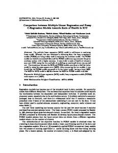
inputs will result in the less accuracy of the estimation (Schaap et al 1998; Amini et al 2005). Input data in Sarmadian et al (2009) study were clay and OC while in the present study, five variables were considered as input data. The scatter plot of the measured against predicted CEC values obtained from the MLR model for the test data set with a poor correlation coefficient is illustrated in Fig. 2. Artificial neural networks (MLP and RBF) In order to predict the soil CEC indirectly through ANN model, as above-mentioned two different algorithms of ANN including radial basis function (RBF) and multi-layer perceptron (MLP) models were used in this study. The input data were those employed by MLR model. In order to this end, all data set were first normalized between 0 and 1 to achieve effective network training. Luk et al (2000) stated that neural networks trained on normalized data, achieve better performance and faster convergence in general, although the advantages diminish as network and sample size become large. Normalizing the data set was done through the Eq. 7:

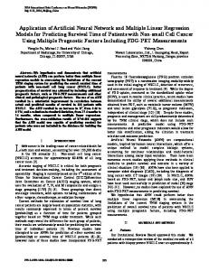
(7) Where xnorm is the normalized value, x is the actual value, xmax is the maximum value and xmin is the minimum value. A three-layered feed-forward ANN architecture with an input layer, one hidden layer and an output layer that is schematically represented in Fig.. 3 were developed for predicting CEC by means of both ANN models in Khuzestan province. A feed-forward network is a common ANN architecture that requires relatively little memory and is generally fast (Lawrence, 1994). The optimal architecture of each network was determined based on R2 and MSE values criteria of the trained data set. Table 5 summarizes the results of statistical performance and optimal architecture of ANN networks. For MLP network, the architecture including five neurons in the input layer and one neuron in the output layer

S.D 29.17 0.23 0.15 3.58 16.56 10.09 9.13 3

B.D gr cm-3

CEC (Cmol kg-1)

1 -0.022

1

with tangent sigmoid transfer function (tansig) at hidden layer consists of three neurons and a linear transfer function (purelin) at output layer gave the best results. The hidden layer with seventy five neurons was identified as an optimal structure for RBF network, while the number of neurons in input and output layers was the same one for MLP. In order to employ RBF, Gaussian function that is the most widely used in applications, was chosen as a Threshold function for hidden layer. The findings of Chen et al (1991) suggested that the choice of radial basis function used in network does not significantly affect performance of network. The MLP and RBF networks fed with three forth of the normalized operational data were trained for 350 and 75 epochs, respectively. In the next step, a regression analysis of the network response between ANN outputs and the corresponding targets was performed. As seen from Table 5, the values of R2 and MSE between ANNs outputs and the corresponding targets indicated that provided predictions using MLP model (R2= 0.83, MSE= 0.008) had higher accuracy than RBF ones (R2= 0.74, MSE= 0.034). The levels of R2 and MSE derived by both ANN models for predicting studied soil CEC had higher and less values, respectively, than those derived by multiple linear regressions which were a support for those previous studies conducted by Tamari et al (1996), Minasny and McBratney (2002), Amini et al (2005), Tekin and Akbas (2011) and other researchers. Amini et al (2005) showed that the neural networks PTFs were more efficient than the regression ones to predict the CEC. This is due to that unlike the traditional regression PTFs, ANNs do not require a priori regression model which relates input and output data that in general is difficult because these models are not known (Schaap and Leij, 1998). Also Tamari et al (1996) and Minasny and McBratney (2002) stated that when the number of input parameters is greater than three, ANNs usually perform better than regression techniques, particularly when uncertainties in the quality of the data were small. Additionally, many investigations have indicated that a neural network with one hidden layer is capable of approximating any finite non-linear function with very high

41

accuracy (Kim and Gilley, 2008; Yimaz and Kaynar, 2011). The scatter plots between experimental and predicted CEC

rules and each fuzzy rule would be constructed using two or more membership functions in layer 2. Several methods have been proposed to classify the input data and to make the rules, among which the most widespread are grid partition and subtractive fuzzy clustering (Aqil et al, 2007; Ertunc and Hosoz, 2008; Yetilmezsoy et al, 2011). In this study, subtractive fuzzy clustering was taken in consideration. The descriptive performance of the ANFIS model for the test data set and the related statistical evolutionary results are given in Fig. 6 and Table 5. The values of 0.5 and 0.009 for R2 and MSE parameters, respectively, for ANFIS testing stage, show approximately similar prediction accuracy of ANFIS model with the MLR, while its efficiency were less than both ANN models. Generally, results of the comparison of MSE and R2 indices for predicting CEC showed that prediction performance of the MLP was more than RBF one, while, their predictive performance had higher accuracy than those of ANFIS and MLR models. This is in line with the work done by Yilmaz and Kaynar (2011). Their findings demonstrated that prediction performances of the ANN models (MLP and RBF) had higher accuracy than both multiple regression equations and adaptive neuro-fuzzy inference system for predicting swell potential of clayey soil. Also, results indicated that the ANFIS model for prediction of CEC had approximately similar accuracy when compared with the multiple regression models. Materials and methods Data collection

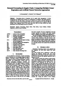
Fig 1. (a) Two input first-order Sugeno fuzzy model with two rules and (b) equivalent ANFIS architecture.

Fig 2. Measured CEC (Cmol/Kg) versus Predicted CEC (Cmol/Kg) using MLR.

using MLP and RBF models with acceptable accuracy are indicated in Figs. 4 and 5, respectively. Adaptive neuro-fuzzy inference system (ANFIS) In this study, ANFIS model was also applied for predicting CEC using the same normalized data that were used for ANN models. In the ANFIS system, each input parameter might be clustered into several class values in layer 1 to build up fuzzy

This study was carried out in Khuzestan province (50◦ 33ʺ N to 47◦ 40ʺ E) located in the south west of Iran. The climate of Khuzestan province varies from arid to humid (Zarasvandi et al, 2011). The determination of numerous chemical and physical properties was carried out on 100 soil samples collected from surface horizons of 100 soil profiles located in Khuzestan Province. Using profile description and laboratory analyses of soil samples, all the studied soils were classified as Entisols and Aridisols on the basis of Soil Survey Staff (2010). The soil properties measured for this study were organic carbon percentage (%OC), calcium carbon content percentage (Caco3), soil salinity (EC), cation exchange capacity (CEC), bulk density (B.D) and soil particle-size distribution. The following analytical methods were employed to measure each of parameters for this study: %OC was determined using Walkley-Black method (Nelson and Sommers, 1982), Particle size distribution using pipette method (Gee and Bauder, 1986), CEC using sodium acetate (pH= 8.2) (Thomas, 1982), EC using EC meter (ISWRI, 1998), B.D using clod method (Blake and Hartge, 1986) and % Caco3 by titration method (ISWRI, 1998). The results of determinations were used as input variables to develop the CEC estimation models. Multiple regression models The general purpose of multiple regressions is to learn more about the relationship between several independent or predictor variables and a dependent or criterion variable. Multiple linear regressions (MLR) are the most common method used in development PTFs. The general form of the regression equations is according to Eq. 1: Y=b0 + b1X1 + ... +b7X7 + b8X8 + … +bnXn (1) Where Y is the dependent variable representing CEC, b0 is the intercept, b1. . .bn are regression coefficients, and X1–Xn are independent variables referring to basic soil properties.

42

Table 3. Coefficients of variables used in MLR models to develop PTFs for prediction CEC. Model Independent variables Coefficient Std. error t-Value Constant 17.012 6.140 2.771 B.D -3.644 1.615 -2.257 Clay 0.144 0.025 5.753 LogEC 0.289 0.337 0.856 1 LnOC 0.822 0.322 2.553 LnSand 0.572 0.428 1.336 -2.931 1.384 -2.117 LnCaCO3 LnSilt 2.016 0.952 2.118 Constant 16.441 6.093 2.698 B.D -3.424 1.591 -2.152 Clay 0.144 0.025 5.756 2 LnOC 0.770 0.316 2.439 LnSand 0.565 0.427 1.323 LnCaCO3 -2.931 1.382 -2.121 LnSilt 2.153 0.936 2.299 Constant 20.852 5.125 4.069 B.D -3.215 1.591 -2.021 Clay 0.122 0.019 6.515 3 LnOC 0.936 0.291 3.217 LnCaCO3 -2.689 1.377 -1.953 LnSilt 1.330 0.703 1.891 Table 4. Performance indices (R2and MSE) for different regression models. Model Predictors 1 Constant, Ln Silt, Clay, Ln OC, B.D, Log EC, Ln Caco3, Ln Sand 2 Constant, Ln Silt, Clay, Ln OC, B.D, Ln Caco3, Ln Sand 3 Constant, Ln Silt, Clay, Ln OC, B.D, Ln Caco3

Sig. Level 0.007 0.027 0.000 0.395 0.013 0.186 0.038 0.038 0.009 0.035 0.000 0.017 0.190 0.037 0.024 0.000 0.047 0.000 0.002 0.055 0.063 R2 0.57 0.57 0.56

MSE 1.14 1.13 1.15

Table 5. Performance indices (R2and MSE) for different models. Model

Architecture

Threshold function

MLR MLP RBF ANFIS

5-3-1 5-75-1

Tansig-Purelin Gaussian

Artificial neural networks (ANNs) Artificial neural networks (ANNs) are a form of artificial intelligence, which, by means of their architecture, attempt is made to simulate the biological structure of the human brain and nervous system (Zurada, 1992; Fausett, 1994). A neural network consists of simple synchronous processing elements, called neurons, which are inspired by biological nerve system (Malinova and Guo, 2004). The mathematical model of a neural network comprises of a set of simple functions linked together by weights. The network consists of a set of input units x, output units y and hidden units z, which link the inputs to outputs. In this study, two different types of ANNs were developed. The first ANN model was multi-layer perceptron which is the most commonly-used neural network structure in ecological modeling and soil science (Agyare, 2007); whereas, the second ANN model was radial basis function. Matlab 7.1 software (2005) was used to develop PTFs for predicting CEC by means of ANN models. Multi-layer perceptron (MLP) Multi-Layer Perceptron has three layers including an input layer, one or more hidden layers and an output layer. Each layer has a number of processing units called neuron (node) and each unit is fully interconnected with weighted connections to units in the subsequent layer. The MLP

Training R2 0.56 0.92 0.77 0.55

Testing MSE 1.15 0.002 0.007 0.009

R2 0.51 0.83 0.74 0.50

MSE 1.21 0.008 0.034 0.009

transforms n inputs to l from the first layer, which are transmitted through the hidden layer, to the output layer by means of some nonlinear functions. In order to find optimal weights by means of MLP, firstly the network is trained using a procedure called error back propagation by observing a large number of input and output examples to develop a useful formula for prediction. The output of the network is determined by the activation of the units in the output layer (Dawson et al, 2006; Yilmaz and Kaynar, 2011). Radial basis function (RBF) The structure of RBF is similar to that of MLP. The main difference between MLP and RBF is that, unlike the MLP, there is only a hidden layer in RBF network which contains nonlinear nodes called RBF units that measure the distance between an input data vector and the center of its RBF (Yilmaz et al, 2011). Training stage in RBF has two steps, firstly, calculating the function’s center and its deviation or width and subsequently, calculating the output weights. There are various ways for selecting the centers and widths of functions such as random subset selection, K-means clustering, orthogonal least squares learning algorithm, and RBF-PLS. In this study, the forward subset selection routine was used to select the centers from training set samples. The adjustment of the connection weight between hidden layer and output layer is performed using a least squares solution

43

Fig 3. Structure of MLP and RBF networks for predicting CEC.

Fig 6. Measured CEC versus predicted CEC (Cmol/Kg) values using ANFIS.

after selecting the centers and width of radial basis functions (Yao, 2002; Yilmaz et al, 2011). Adaptive neuro-fuzzy inference system (ANFIS) model

Fig 4. Measured versus predicted CEC values using MLP network.

An adaptive network, as its name implies, is a network structure consisting of nodes and directional links through which the nodes are connected. Moreover, parts or all of the nodes are adaptive, which means each output of these nodes depends on the parameters pertaining to this node and the learning rule specifies how these parameters should be changed to minimize a prescribed error measure (Jange, 1993). In ANFIS, fuzzy rule bases are combined with neural networks to train the system using experimental data and obtain appropriate membership functions for process prediction and control (Lertworasirikul, 2008). Takagi– Sugeno–Kang (TSK) model (Takagi and Sugeno, 1985) that is one of the most frequently-used precise fuzzy models was used in the current study to predict soil CEC. In order to simplify, it is assumed that the inference system has two input variables x and y as each variable has two fuzzy subsets .A typical rule set with two fuzzy if–then rule set for a first-order Sugeno fuzzy model can be defined as Eq. 2 and 3: Rule 1: If x is A1 and y is B1

Then f1 = p1x + q1y + r1

Rule 2: If x is A2 and y is B2

(2) Then f 2 = p2x + q2y + r2 (3)

Fig 5. Measured versus predicted CEC values using RBF network.

Where A1, A2 and B1, B2 are the MFs for inputs x and y respectively, p1, q1, r1 and p2, q2, r2 are the parameters of the output function. The corresponding equivalent ANFIS architecture for two input variable first-order Sugeno fuzzy model with two rules is illustrated in Fig. 1(a). The general architecture of ANFIS consists of five layers, namely, a fuzzy layer, a product layer, a normalized layer, a defuzzy layer and a total output layer is depicted in Fig. 1(b). In this architecture, the circular nodes represent nodes that are fixed, whereas the square nodes are nodes that have parameters to be learnt. Layer 1: Every node in this layer is represented by a square node including a node function. The node function employed

44

by each node determines the membership relation between the input and output functions. Layer 2: every node in this layer is a fixed (circle) labeled II node and its output is produced by signals obtained from layer 1. Layer 3: every node in this layer is a fixed (circle) node labeled N. The nodes normalize the firing strength by calculating the ratio of firing strength for this node to the sum of all the firing strengths. Layer 4: Every node in this layer is represented by a square node including a node function. Layer 5: The single node in this layer is a fixed (circle) node labeled Ʃ that computes the overall output as the summation of all incoming signals. Performance evaluation criteria Two different types of standard statistical performance evaluation criteria were used to control the accuracy of the prediction capacity of the models developed. These are mean square error (MSE) and the determination coefficient (R2). The two performance evaluation criteria used in the current study can be calculated using Eq. 4 and 5:

(4)

(5) Where N is the number of data, yi is the measured value of each variable, is the predicted value of each variable and is the average of predicted value of each variable. Conclusion In this study, an attempt has been made to analyze and compare multiple linear regressions (MLR), adaptive neurofuzzy inference system (ANFIS) and artificial neural network (ANN) including multi-layer perceptron (MLP) and radial basis function (RBF) models to develop pedo-transfer function for predicting soil cation exchange capacity by using available soil properties. The statistical prediction performances of used models are measured in terms of correlation coefficient (R2) and mean square error (MSE). The results of prediction CEC indicated that the measured correlation coefficient between predicted and observed data using equation obtained from the MLR and ANFIS models were approximately similar and very poor. The MLP model for prediction of CEC revealed the most reliable prediction when compared with the other models. Also, descriptive performance indices (R2 and MSE) between predicted and experimental data for RBF model showed higher accuracy comparing with both ANFIS and MLR models. Consequently, with the use of proposed ANNs especially, MLP network, the performance of CEC condensers can be determined by performing only a limited number of test operations, thus saving engineering effort, time and funds. References Agyare WA, Park SJ, Vlek PLG (2007) Artificial neural network estimation of saturated hydraulic conductivity. Vadose Zone J. 6: 423–431

Amini M, Abbaspour KC, Khademi H, Fathianpour N, Afyuni M, Schulin R (2005) Neural network models to predict cation exchange capacity in arid regions of Iran. Eur J Soil Sci. 56: 551-559 Aqil M, Kita I, Yano A, Nishiyama S (2007) A comparative study of artificial neural networks and neuro-fuzzy in continuous modeling of the daily and hourly behaviour of runoff. J Hydrol. 337: 22–34 Blake GR, Hartge KH (1986) Bulk density. In: Klute, A. (Ed.). Methods of Soil Analysis. Part 1, second ed. Agron. Monogr. 9. ASA and SSSA, Madison, WI, pp: 363-375 Bouma J (1989) Using soil survey data for quantitative land evaluation. Adv Soil S. 9: 177-213 Caravaca F, Lax A, Albaladejo J (1999) Organic matter, nutrient contents and cation exchange capacity in fine fractions from semiarid calcareous soils. Geoderma. 93: 161–176 Carpena O, Lux A, vahtras K (1972) Determination of exchangeable calcareous soils. Soil Sci. 33: 194-199 Chen S, Cowan CFN, Grant PM (1991) Orthogonal least squares learning algorithm for radial basis function networks. IEEE Trans Neural Netw. 2(2):302–309 Christidis GE (1998) Physical and chemical properties of some bentonite deposits of Kimolos Island, Greece. Appl Clay Sci. 13(2): 79–98 Dawson CW, Abrahart RJ, Shamseldin AY, Wilby RI (2006) Flood estimation at ungauged sites using artificial neural networks. J Hydrol. 319: 391–409 Ertunc Hm, Hosoz M (2008) Comparative analysis of an evaporative condenser using artificial neural network and adaptive neuro-fuzzy inference system. Int J Refrig. 31: 1426-1436 Evans LJ (1989) Chemistry of metal retention by soils. Environ Sci Technol. 23: 1046–056 Fausett LV (1994) Fundamentals of neural networks: Architecture, algorithms, and applications, Prentice-Hall, Englewood Cliffs Francois M, Dubourguier HC, Li D, Douay F (2004) Prediction of heavy metal solubility in agricultural topsoils around two smelters by the physico-chemical parameters of the soil. Aquat Sci. 66: 78–85 Gee GW, Bauder JW (1986) Particle size analysis. Pp. 383411. In: A. Klute (Ed.), Methods of Soil Analaysis. Part 1.Amrican society of Agronomy, Madison, Wisconsin, USA Gokceoglu C, Zorlu K (2004) A fuzzy model to predict the uniaxial compressive strength and the modulus of elasticity of a problematic rock. Eng Appl Artific Intel. 17:61–72 Horn AL, Düring RA, Gath S (2005) Comparison of the prediction efficiency of two pedotransfer functions for soil cation exchange capacity. J Plant Nutr Soil Sci. 168: 372374 Igwe CA, Nkemakosi JT (2007) Nutrient element contents and cation exchange capacity in fine fractions of southeastern nigerian soils in relation to their stability. Commun Soil Sci Plan. 38: 1221-1242 Iranian Soil and Water Research Institute (ISWRI) (1998) Tehran, Iran. Soil Bulletin. 758: 83-102 (In Persian) Jange J-SR (1993) ANFIS: adaptive-network-based fuzzy inference system. IEEE Trans Syst Man Cybern. 23(3): 85665 Jung WK, Kitchen NR, Sudduth KA, Anderson SH (2006) Spatial characteristics of claypan soil properties in an agricultural field. Soil Sci Soc Am J. 70: 1387-1397 Keshavarzi A, Fereydoon Sarmadian1 F, Abbas Ahmadi, A (2011). Spatially-based model of land suitability analysis using Block Kriging. Aust J Crop Sci. 5(12):1533-1541

45

Keshavarzi A, Sarmadian F, Rahmani A, Ahmadi A, Labbafi R, Iqbal MA (2012) Fuzzy Clustering Analysis for Modeling of Soil Cation Exchange Capacity. Aust J agric eng. 3(1):27-33 Kim M, Gilley JE (2008) Artificial Neural Network estimation of soil erosion and nutrient concentrations in runoff from land application areas. Comput Electron Agric. 64: 268–275 Lawrence J (1994) Introduction to Neural Networks. California Scientific Software Press, Nevada City, CA Lertworasirikul S (2008) Drying kinetics of semi-finished cassava crackers: a comparative study. LWT – Food Sci Technol. 41: 1360–1371 Luk, K.C., Ball, J.E., Sharma, A., 2000. A study of optimal model lag and spatial inputs to artificial neural network for rainfall forecasting. J Hydrol. 227: 56–65 Malinova T, Guo ZX (2004) Artificial neural network modeling of hydrogen storage properties of Mg-based Alloys. Mater Sci Eng. 365: 219–227 Manrique LA, Jones CA, Dyke PT (1991) Predicting cation exchange capacity from soil physical andchemical properties. Soil Sci Soc Am J. 55: 787-794 Matlab 7.1 (2005) Software for technical computing and Model-Based Design. The Math Works Inc Matula J (2009) A relationship between multi-nutrient soil tests (Mehlich 3, ammonium acetate, and water extraction) and bioavailability of nutrients from soils for barley. Plant Soil Environ. 55(4): 173–180 Merdun H, Cinar O, Meral R, Apan M (2006) Comparison of artificial neural network and regression pedotransfer functions for prediction of soil water retention and saturated hydraulic conductivity. Soil Till Res. 90: 108–116 Minasny B, McBratney AB (2002) Theneuro-m method for fitting neural network parametric pedotransfer functions. Soil Sci Soc Am J. 66: 352–361 Nelson DW, Sommers LE (1982) Total carbon, organic carbon, and organic matter. In: Page, AL, Miller, RH, Keeney DR (Eds.), Methods of Soil Analysis. Part II, 2nd ed. American Society of Agronomy, Madison, WI, USA. pp. 539-580 Sarmadian F, Taghizadeh Mehrjardi R, Akbarzadeh A (2009) Modeling of some soil properties using artificial neural network and multivariate regression in Gorgan province, north of Iran. Aust J Basic Appl Sci. 3(1): 323-329 Schaap MG, Leij FJ, van Genuchten MTh (1998) Neural networkanalysis for hierarchical prediction of soil hydraulic properties. Soil Sci Soc Am J. 62: 847–855 Schaap MG, LeijFJ (1998) Using neural networks to predict soilwater retention and soil hydraulic conductivity. Soil Till Res. 47 :37–42 Seybold CA, Grossman RB, Reinsch TG (2005) Predicting Cation Exchange Capacity for Soil Survey Using Linear Models. Soil Sci Soc Am J. 69: 856-86 Sposito G (1989) The chemistry of soils. Oxford University Press. 277pp

Takagi T, Sugeno M (1985) Fuzzy identification of systems and its applications to modeling and control. IEEE Trans Syst Man Cybern. 15: 116–132 Tamari S, Wösten JHM, Ruiz-Suárez JC (1996) Testing an artificial neural network for predicting soil hydraulic conductivity. Soil Sci Soc Am J. 60: 1732–1741 Tang L, Zeng G, Nourbakhsh F, Guoli L, Shen GL (2009) Artificial Neural Network Approach for Predicting Cation Exchange Capacity in Soil Based on Physico-Chemical Properties. Environ Eng Sci. 26(1): 137-146 Tekin E, Akbas SO (2011) Artificial neural networks approach for estimating the groutability of granular soils with cement-based grouts. B Eng Geol Environ. 70:153– 161 Thomas GW (1982) Exchangeable cation. In: Page, A. L. (Ed.), Method of soil analysis. part2. Agron. Monograph 9, ASA, WI: 159-165 USDA (2010) Soil Survey Staff.Keys to Soil Taxonomy.11th edition Wosten JHM, Finke PA, Jansen MJW (1995) Comparison of class and continuous pedotransfer functions to generate soil hydraulic characteristics. Geoderma. 66:227–237 Yao X, Xiaoyun Z (2002) Radial basis function neural network based QSPR for the prediction of critical pressures of substituted benzenes. Comput Chem. 26: 159–169 Yetilmezsoy K, Fingas M Fieldhouse, B (2011) an adaptive neuro-fuzzy approach for modeling of water-in-oil emulsion formation. Colloids Surf A Physicochem Eng Aspect. 389: 50– 62 YetilmezsoyK,Demirel S (2008) Artificial neural network (ANN) approach for modeling of Pb(II) adsorption from aqueous solution by Antep pistachio (Pistacia Vera L.) shells. J Hazard Mater. 153: 1288–1300 Yilmaz I, Kaynar O (2011) Multiple regression, ANN (RBF, MLP) and ANFIS models for prediction of swell potential of clayey soils. Expert Syst Appl. 38: 5958–5966 Yilmaz I, Marschalko M, Bednarik M, Kaynar O, Fojtova, L (2011) Neural computing models for prediction of permeability coefficient of coarse-grained soils. Neural Compu & Applic. DOI: 10.1007/s00521-011-0535-4 Zarasvandi A, Carranza EJM, Moore F, Rastmanesh F (2011) Spatio-temporal occurrences and mineralogical– geochemical characteristics of airborne dusts in Khuzestan Province (southwestern Iran). J Geochem Explor. 111: 138–151 Zorluer I, Icaga Y, Yurtcu S, Tosun H (2010) Application of a fuzzy rule-based method for the determination of clay dispersibility. Geoderma. 160: 189–196 Zurada JM (1992) Introduction to artificial neural systems, West, St. Paul, Minnesota

46