Comparing Multiple Linear Regression and Artificial ...

International Review on Modelling and Simulations (I.RE.MO.S.), Vol. xx, n. x June 2008

Demand Forecasting in Supply Chain: Comparing Multiple Linear Regression and Artificial Neural Networks Approaches S. Benkachcha1, J. Benhra2, H. El Hassani3 Abstract – Forecasting plays an important role in supply chain management. It allows anticipating and meeting future demands and expectations of customers. This paper presents a contribution that will shed light on ways how to improve the quality of forecasts through the application of Artificial Neural Networks (ANNs). The neural network model is compared with the multiple linear regression (MLR). The results show that ANNs are more efficient and more promising as far as forecasting accuracy is concerned.

Keywords: Demand Forecasting, Supply Chain, Time Series, Causal Method, Multiple Regression, Artificial Neural Networks.

Nomenclature ANN(s) MLR MLP LM

= = = =

GDA

=

BR SSE SSR SST MSE RMSE MAE MAPE

= = = = = = = =

Artificial Neural Network(s); Multiple Linear Regression; Multilayer Perceptron; Levenberg -Marquardt back propagation algorithm; Gradient descent with adaptive learning rate back propagation; Bayesian regulation back propagation; Error Sum of Squares; Regression Sum of Squares; Total Sum of Squares; Mean Square Error; Root Mean Square Error; Mean Absolute Error; Mean Absolute Percentage Error

I.

Introduction

In any production environment, demand forecasting plays an important role for managing integrated logistics systems. It provides valuable information for several basic logistics activities including purchasing, inventory management, and transportation. Actually there are extensive forecasting techniques available for anticipating the future. This paper attempts to contribute to the improvement of the quality of forecasts by using Artificial Neural Networks. It discusses two methods of dealing with demand variability. First linear multiple regression is used as a causal method to determine the relationship between forecast variable and causal variables. The regression model is then used to forecast future demand. Secondly a multilayer perceptron (MLP) is used to model the relationship between the same set of input and output variables. The Artificial Neural Network (ANN) is trained for different structures, and several learning rules are used to make sure the ANN weights

have been evaluated. The best configuration and most accurate algorithm are retained. The neural network model is compared to the multiple linear regression [1]. The rest of the paper is organized as follows. Section 2 will review the literature in forecasting and the use of Artificial Neural Networks in this area. Section 3 will present two prediction models: multiple linear regression method and Artificial Neural Network model. Section 4 will discuss the results obtained using this methodology in a case study. Section 5 will consist of the conclusion of the paper.

II.

Literature review

Quantitative forecasting models can be gathered into two categories: the time series models and causal methods. Time series analysis tries to determine a model that explains the historical demand data and allows extrapolation into the future to provide a forecast in the belief that the demand data represent experience that is repeated over time. This category includes naïve method, moving average, trend curve analysis, exponential smoothing, and the autoregressive integrated moving averages models. The reasons for their popularity are that they are cost effective, easy to develop and implement so times series models are appreciated for they have also been used in many applications such as: Economic Forecasting, Sales Forecasting, Budgetary Analysis, Stock Market Analysis, Process and Quality Control and Inventory Studies [2]. On the one hand these techniques are appropriate when we can describe the general patterns or tendencies, without regard to the factors affecting the variable to be forecast [3]-[4]. On the other hand, the causal methods are used to look for potential and pertinent demand reasons, when a set of variables affecting the situation are available [5]. Among the models of this category,

Manuscript received and revised May 2008, accepted June 2008

Copyright © 2008 Praise Worthy Prize S.r.l. - All rights reserved

F. A. Author, S. B. Author, T. C. Author

multiple linear regression uses a predictive causal model that identifies the causal relationships between the predictive (forecast) variable and a set of predictors (causal factors). For example, the customer demand can be predicted through a set of causal factors such as predictor’s product price, advertising costs, sales promotion, seasonality, etc. [6]. Both kinds of models (time series models and the linear causal methods) are easy to develop and implement. However they may not be able to capture the nonlinear pattern in data. Neural Network modelling is a promising alternative to overcome these limitations [7]. C.A.Mitrea, M.C. K. Lee, and Z.Wu, compared different forecasting methods like moving average and autoregressive integrated moving average with ANN models as Feed-forward neural network and nonlinear autoregressive network with exogenous inputs [8]. The results have shown that forecasting with ANN offers better predictive performances. M. M. Tripathi , K. G. Upadhyay and S. N. Singh, have used a General Regression Neural Network (GRNN) computing technique for predicting day-ahead electricity prices in the PJM market. The obtained results confirm the efficiency and the accuracy of the proposed method [9]. After being properly configured and tried by historical data, ANN can be used to approximate accurately any measurable function. Because they are fast and accurate, several researchers use ANNs to solve problems related to demand forecasting. The idea behind this approach is to identify patterns hidden among data and make generalizations of these patterns. ANNs provides outstanding results even in the presence of noise or missing information [10].

relationship with the dependent variable, but also by the availability of the data describing their historical [11]. III.1.1. Simple linear regression model The simple linear regression model can be written as follows

yi  0  1 xi   i

(1)

Where the response variable yi is modeled as a linear combination of the predictor xi , plus a random error  i . To fit the model to the data, the least-squares solution gives the smallest possible sum of squared deviations of the observed yi . Let ˆ0 and ˆ1 be numerical estimates of the unknown coefficients  0 and 1 . The estimated response is given by substituting the estimates for the parameters in equation (1):

yî  ˆ0  ˆ1 xi

(2)

The least squares fitting process gives ˆ0 and ˆ1 that minimize the error sum of squares: n

n

i 1

i 1

SSE   ( yi  yî ) 2   ei2 Where :

(3)

ei  ( yi  yî ) is the observed residual for the

ith observation [11]. Differentiating SSE with respect to each parameter, and setting the results equal to zero, gives two equations, in two unknowns, called the normal equations:

n  ˆ0     xi  ˆ1



  x  ˆ    x  ˆ

III. Methodology

i

2 i

0

Solving for ˆ1 :

III.1. Linear Regression Approach

ˆ1 

Causal methods involve the establishment, based on past data, of a relationship between the variable to predict (dependent variable) and the one or more independent variables (explanatory variables). Variables can be either internal to the company or related to the economy and competition. This approach presupposes a common sense analysis of the reality of causality between variables, without which any correlation could be only a temporary phenomenon due to chance. Among these methods, regression techniques are well used to forecast the short and medium term. They are interesting when products are influenced by factors on which data is available historically and for the forecast period. There are two types of linear regression analysis: simple and multiple: the simple linear regression is composed of a dependent variable and an independent variable while the multiple linear regression analysis involves two or more independent variables. The choice of these variables must be justified by their strong

n xi yi   xi  yi n x    xi  2 i

2



1



y x y i

i

i

(4)

 ( x  x )( y  y )  (x  x ) i

i

2

(5)

i

Solving for ˆ0 using the ˆ1 value:

1 (6) n Where x and y are the averages of observations xi and yi respectively [11].

ˆ0  ( yi  ˆ1  xi )  y  ˆ1 x

III.1.2. Multiple linear regression model The general multiple linear regression model, [12]-[13], can be represented as follows: yi  0  1 xi1   2 xi 2  ...   p xip   i (7) Where for each observation i  1,....., n, there are:


International Review on Modelling and Simulations, Vol. x, N. x


The fitted or predicted values are

p predictor variables xi1 , xi 2 ,...., xip ;



p  p  1 parameters  0 , 1 ,  2 ,....,  p to be estimated;

yˆ   X  b   X   X   X 

 i is the ith error term.

yˆ   H  y

Using linear algebra notation, the model can be compactly written :

y  X     n p p1

nx1

n1

x11 x21 x31 xn1

xn 2

-

y is the

(13) T

The unknown vector of coefficients  of the model is estimated by the least squares method, which minimizes the “residual sum of squares,” (PA Cornillon and E. Matzner-Løber, 2010).

 y X  

Q     2  X 

 y  X    0

T

(14)

(9)

Hidden Layer

Output Layer

Data Output

y   X   is zero.

T

is the hat

Data Input

Input Layer

The minimum occurs where the gradient vector of the

  y  X  

T

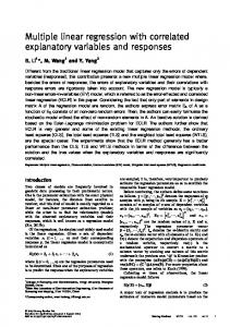
Feed forward neural networks allow only unidirectional signal flow. Furthermore, most feed forward neural networks are organized in layers and this architecture is often known as MLP (multilayer perceptron) [16]. An example of feed forward neural network is shown in figure 1. It consists of an input layer, a hidden layer, and an output layer.

-  is the p 1 vector of parameters to be estimated; -  is the n1 vector of error terms.

2

1

III.2.1. Feed forward Neural Networks

 X  is the n  p design matrix for the model;

Q   y  X 

y

III.2. Artificial Neural Networks Approach

n1 column vector of responses;

squared length of

T

e  y  yˆ  1   H  y

Where: -

X 

The residual values are defined as the differences between the response and the fit to the response data.

x1 p    0  1  x2 p   1   2    x3 p     3    3            xnp    p   n 

x12 x22 x32

1

matrix.

Or:

 y1  1  y  1  2   y3   1        y  1  n 



 H    X   X   X   X 

Where

(8)

T

(10) Fig.1 Basic structure of Multilayer Perceptron

Giving a set of linear equations, called the “normal equations” to be solved for  .

X  X   X  T

T

y

Each node in a neural network is a processing unit which contains a weight and summing function followed by a non-linearity Fig. 2.

(11)

x1

The solution is a vector ˆ which estimates the unknown vector of coefficients  .



ˆ   X   X  T



1

X 

T

y

12

wi1

x2

wi 2

x3

wi 3

…. .

… .

∑ f

oi

wiN

xN Fig.2 Single neuron with N inputs. Copyright © 2008 Praise Worthy Prize S.r.l. - All rights reserved



18 19 20 21 22

The computation related with this neuron is described below: N

oi  f ( wij x j )

(15)

20783 21917 20878 21508 22261

12419 13265 13173 13211 14070

40152 65490 37639 19425 45300

74915 81030 86686 97088 108739

j 1

oi is the output of the neuron i , f ( ) is the transfer function, wij is the connection weight between Where

neuron

IV.1. Multiple linear regression model implementation

j and neuron i and x j is the input signal from

IV.1.1. Determination of the parameters

neuron j .

The fitted regression equation is: yî  0  1 xi1   2 xi 2  3 xi 3

The general process responsible for training the network is mainly composed of three steps: feed forwarding the input signal, back propagating the error and adjusting the weights. The back-propagation algorithm tries to improve the performance of the neural network by reducing the total error which can be calculated by:

SE 

2 1 o jp  d jp   2 p j

Where the Estimated Coefficients are given in table 2: TABLE II ESTIMATED COEFFICIENTS OF THE REGRESSION MODEL

Coefficient β0 β1 β2 β3

(16)

Where: - SE is the square error, - p is the number of applied patterns,

Value -31823,53 2,41 5,70 -0,17

The fitted or predicted response values are given by the estimated model:

yˆ

th

-

d jp is the desired output for j neuron when p

-

o jp is the jth neuron output.

th

                

pattern is applied and

IV. Approach Implementation and Discussion The study is based on a data set used to predict future sales of a product (y) based on advertising spending (x1), promotional expenses (x2) and quarterly sales of its main competitor (x3) [1]. For this we have 22 observations of three sets of input and output series shown in Table 1.

x1

x2

x3

y

4949 5369 6149 6655 8114 8447 10472 10508 11534 12719 13743 16168 16035 16112 18861 19270 21536

7409 7903 9289 9914 8193 8711 9453 9194 10149 10403 10806 11557 11092 10979 12117 11319 12702

43500 20209 47640 34563 36581 52206 76788 42107 78902 73284 61871 85265 28585 26921 94457 17489 99820

16793 22455 25900 25591 34396 38676 34608 35271 39132 46594 57023 59720 62805 61905 65963 72869 71963



15002   22786   27919     34925   28289      82372     85635   87328     92156     94483  

 b

X    1 1 1 1 1

4949 5369 6149 6655 8114

7409 7903 9289 9914 8193

1 1 1 1 1

20783 21917 20878 21508 22261

12419 13265 13173 13211 14070

43500  20209  47640   34563   31823,53  36581   2, 41    5, 70 40152       0,17  65490  37639   19425   45300 

The fitted curve provides a first visual examination to evaluate the efficiency of the fitting with the linear regression model.

TABLE I DATA SET FOR REGRESSION AND ANN MODELS N° 1 2 3 4 5 6 7 8 9 10 11 12 13 14 15 16 17

(17)

Fig.3 Fitted response with multiple linear regression model




Overall we can say that the model is good, since the estimated response curve approximately follows the curve of the observed responses. The following figure illustrates the regression analysis between the fitted response and the corresponding targets (observed responses).

The residuals (plotted as open circles) appear randomly scattered around zero. In fact, a property of the model is that the sum of the residuals is zero when the model includes the constant term  0 [11]. The R2 (R-square) measure is used to evaluate the performance of regression analysis. This statistic is defined as the ratio of the explained to the total variation [14]-[15]:

R2 

SSR SSE  1 SST SST

Where: - SSR is the regression sum of squares (Explained Variation) n

SSR    yî  y 

2

i 1

- SST is the total sum of squares (Total Variation) n

SST    yi  y 

2

i 1

- SSE is the error sum of squares (Unexplained Variation)

Fig.4 Regression outputs versus the targets

The outputs are plotted versus the targets as open circles. The best linear fit is indicated by a dashed line. The perfect fit (output equal to targets) is indicated by the solid line. In this example, it is difficult to distinguish the best linear fit line from the perfect fit line because the fit is so good.

n

SSE    yi  yî 

2

i 1

The R-square for this case study is valued at R2  0.9558 . This demonstrates that the linear regression model predicts 95.58% of the variance in the response variable y .

IV.1.2. Evaluating the accuracy of the regression model The ith residue observed value value yˆ i :

IV.2. Neural Network Model implementation

ei is the difference between the

Neural Network Toolbox provides a complete environment to design, train, visualize, and simulate neural networks. The neural network architecture is composed of input nodes (corresponding to the independent or predictor variables x1, x2 and x3), one output node, and an appropriate number of hidden nodes. The most common approach to select the optimal number of the hidden nodes is via experiment or by trial-anderror [17]. One other network design decision includes the selection of activation functions, the training algorithm, learning rate and performance measures. For non-linear prediction problem, a sigmoid function at the hidden layer, and the linear function in the output layer are generally used.

yi and the corresponding adjusted

ei  yi  yî

The scatterplot of residuals is obtained around their mean zero.

Fig.5 scatterplot of residuals Copyright © 2008 Praise Worthy Prize S.r.l. - All rights reserved



x1

y

x2

x3

Fig.6 Multi-layer perceptron model (with Causal variables)

To determine the optimal MLP topology and training algorithm, the mean squares error (MSE) of the ANN is used. It is defined as follows:

Fig.7. ANN trained with Gradient descent with adaptive learning rate back propagation algorithm (GDA)

MSE  SSE (n  p) Where: - SSE is the summed square of residuals - n is the number of observations - p is the number of terms currently included in the model. RMSE alternative

for root mean square error is another of expressing the MSE:

RMSE  SSE (n  p) The results obtained by training several architectures with Levenberg-Marquardt (LM) back propagation algorithm are given in table below: TABLE III PERFORMANCE OF THE ANN TRAINED WITH LM ALGORITHM

neurons in hidden layer 3 neurons

SSE

MSE

RMSE

2,56E+08

1,42E+07

3,77E+03

5 neurons

1,46E+08

8,11E+06

2,85E+03

7 neurons

1,18E+09

6,55E+07

8,09E+03

Fig.8. ANN trained with Levenberg-Marquardt back propagation Algorithm (LM)

It is clearly that an ANN with 5 neurons in the hidden layer gives better fitted response when it is trained by an LM algorithm. Two other learning algorithms are tested by adopting several neural network configuration. These are: - Gradient descent with adaptive learning rate back propagation (GDA): ‘traingda’ function in MATLAB toolbox. - Bayesian regulation back propagation (BR) : ‘trainbr’ training function in MATLAB toolbox. The results are shown in the figures below: Fig.9. ANN trained with Bayesian regulation back propagation Algorithm (BR) Copyright © 2008 Praise Worthy Prize S.r.l. - All rights reserved



The GDA algorithm is not suitable for this case study since a divergence in results is observed. Even if the GDA algorithm uses a dynamic learning coefficient, its performance remains lower than LM, which takes as propagation algorithm a second order function and can estimate the learning rate in each direction of gradient using Hussian matrix [18]. But the comparison between LM and BR algorithms apparently shows the excellence of the Bayesian algorithm, the performance of which does not change by varying the number of neurons in the hidden layer. Calculating the statistics error allows to refine this comparison. The table below shows the values of statics MSE and RMSE for LM algorithm and the BR algorithm. The number of nodes in the hidden layer for the NNt trained with LM algorithm is 5 neurons. Whereas for the BR algorithm this number is indifferent, three, five or seven nodes.

The values obtained for MAE and MAPE shows that the neural model is more efficient than the multiple linear regression model. This is also proved by the following plot.

TABLE IV COMPARISON BETWEEN LM AND BR ALGORITHM TRAINING

Training algorithm LM

SSE

MSE

RMSE

1,46E+08

8,11E+06

2,85E+03

BR

2,09E+08

1,16E+07

3,41E+03

Fig.10 Comparing Artificial Neural Network and Multiple Linear Regression forecast models

By analogy with neural networks, linear regression can be seen as a weighted sum of the inputs: yî  0  1 xi1   2 xi 2  3 xi 3

The results suggest that, with a judicious choice of the architecture, the best training algorithm is the LevenbergMarquardt back propagation algorithm. This is further approved when the time parameter is considered. Indeed, the execution time with LM algorithm is far less than that required by a BR algorithm.

1

xi 2

Mean Absolute Error (MAE) and Mean Absolute Percentage Error (MAPE), are employed as performance indicators in order to measure forecasting performance of proposed neural network model in comparison with multiple linear regression model [15]. Mean Absolute Error is defined as:

2 3

Fig.11 Linear regression visualized as a graph

As a result neural networks provide more flexibility by adding intermediate layers (hidden) containers more than a single node as in the case of regression. Neural networks also have transfer functions assigned to each neuron that captures the non-linearity which characterizes the relationship of inputs to the output as is the case of demand forecasts.

Mean Absolute Percentage Error is defined as:

1 n yi  yî 1 n ei    n i 1 yi n i 1 yi

V.

MAE

MAPE

3,91E+03

0,0813

1,694E+03

0,0456

CONCLUSION

Demand forecasting plays an important role in the supply chain of today’s companies. This article has discussed two causal methods in order to improve the quality of forecasts. First the multiple linear regression has been used to estimate fitted response. Second, a feed forward neural network model has been proposed. The ANN is trained for different structures and several learning rules have been evaluated. The best model of ANN is retained. The results show that ANNs are more

TABLE V COMPARISON BETWEEN ARTIFICIAL NEURAL NETWORK AND MULTIPLE LINEAR REGRESSION

Forecasting Model Multiple Linear Regression Neural Network

yˆ i

xi 3

1 n 1 n ˆ y  y  ei  i i n n i 1 i 1

MAPE 



1

xi1

IV.3. Comparing Artificial Neural Network and Multiple Linear Regression

MAE 

0




[17] G. Zhang, B. E. Patuwo, and M.Y. Hu, Forecasting with artificial

efficient and are very promising for solving forecast problems. This is due to the neural network’s ability of capturing nonlinear and time-varying nature of demand.

neural networks : The state of the art, International Journal of Forecasting.Vol.14, , p 35–62, 1998.

[18] B. M.Wilamowski, H.Yu, Improved Computation for Levenberg Marquardt Training, IEEE Trans. on Neural Networks, vol. 21, no. 6, pp. 930-937, 2010.

References [1] Benkachcha. S, Benhra. J, El Hassani. H, Causal Method and

Authors’ information

Time Series Forecasting model based on Artificial Neural Network, International Journal of Computer Applications (0975 – 8887). Volume 75– No.7, 2013.

1

Said Benkachcha received his DESA in Laboratory of Mechanics of Structures and Materials, LMSM, of ENSEM – Casablanca in 2006. In 2011 He joined the Laboratory of Computer Systems and Renewable Energy (LISER) of the ENSEM Hassan II University, Casablanca, Morocco. His current research field is demand forecasting and collaborative warehouse management.

[2] V.Gosasang , W.Chan., and S.KIATTISIN, A Comparison of Traditional and Neural Networks Forecasting Techniques for Container Throughput at Bangkok Port, The Asian Journal of Shipping and Logistics, Vol. 27, N° 3, pp. 463-482, 2011.

[3] J. S. Armstrong, & K. C. Green, Demand forecasting: Evidencebased methods, Monash University Department of Econometrics and Business Statistics, Working Paper 24-05, 2005.

[4] D. D. Illeperuma, T. Rupasinghe, Applicability of Forecasting Models and Techniques for Stationery Business:A Case Study from Sri Lanka, International Journal of Engineering Research. Volume No.2, Issue No. 7, pp : 449-451, 2013.

2

Jamal BENHRA received his PhD in Automatic and Production Engineering from National Higher School of Electricity and Mechanics (ENSEM), Casablanca in 2007. He has his Habilitation to drive Researchs in Industrial Engineering from Science and Technology University, SETTAT in 2011. He is Professor and responsible of Industrial Engineering Department in National Higher School of Electricity and Mechanics (ENSEM), Hassan II University, Casablanca, Morocco. His current main research interests concern Modeling, Robot, Optimization, Meta-heuristic, and Supply Chain Management.

[5] J. S. Armstrong, Illusions in Regression Analysis, International Journal of Forecasting, Vol.28, p 689 – 694, 2012.

[6] Charles W. Chase Jr., Integrating Market Response Models in Sales Forecasting, The Journal of Business Forecasting. Spring: 2, 27, 1997.

[7] K.Y. Chen, Combining linear and nonlinear model in forecasting tourism demand, Expert Systems with Applications, Vol.38, p 10368–10376, 2011.

[8] C. A. Mitrea, , C. K. M. Lee, and Z. Wu, A Comparison between Neural Networks and Traditional Forecasting Methods: A Case Study, International Journal of Engineering Business Management, Vol. 1, No. 2, p 19-24, 2009.

3

EL HASSANI Hicham received his engineer degree of Industrial Engineering in the National School of applied sciences in 2009. In 2011 He joined the Laboratory of Computer Systems and Renewable Energy (LISER) of the ENSEM Hassan II University, Casablanca, Morocco. His current research field is Modeling, Simulation and Optimization of global supply chain including environmental concerns and reverse logistic.

[9] M. M. Tripathi, K. G. Upadhyay, S. N. Singh, Electricity Price Forecasting using General Regression Neural network (GRNN) for PJM Electricity Market, International Review of Modeling and Simulation (IREMOS),Volume 1, No. 2, pp 318-324, December 2008.

[10] Daniel Ortiz-Arroyo, Morten K. Skov and Quang Huynh, Accurate Electricity Load Forecasting With Artificial Neural Networks , Proceedings of the International Conference on Computational Intelligence for Modelling, Control and Automation, and International Conference on Intelligent Agents, Web Technologies and Internet Commerce (CIMCAIAWTIC’05) , 2005.

[11] Daryl S. Paulson, Handbook of Regression and Modeling Applications for the Clinical and Pharmaceutical Industries (Publisher: Boca Raton : Taylor & Francis Group, LLC, 2007).

[12] John O. Rawlings, Sastry G. Pantula, David A. Dickey, Applied Regression Analysis: A Research Tool (Springer texts in statistics, 2nd ed. p. cm. 1998).

[13] S.Weisberg, Applied Linear Regression (Published by John Wiley & Sons, Inc., Hoboken, New Jersey, 3rd ed. 2005).

[14] S.Makridakis, Accuracy measures: theoretical and practical concerns, International Journal of Forecasting 9, 527-52, 1993.

[15] S. Makridakis, & M. Hibon, Evaluating Accuracy (or Error) Measures, Working Paper, INSEAD, Fontainebleau, France, 1995.

[16] B. M.Wilamowski, Neural Network Architectures. Industrial Electronics Handbook (vol. 5 – Intelligent Systems, 2nd Edition, chapter 6, pp. 6-1 to 6-17, CRC Press, 2011).

