SAMPLING THEORY IN SIGNAL AND IMAGE PROCESSING c 2003 SAMPLING PUBLISHING
Vol. 1, No. 1, Jan. 2002, pp. 0-50 ISSN: 1530-6429
Comparison of numerical methods for the computation of energy spectra in 2D turbulence. Part I: Direct methods Ch.H. Bruneau, P. Fischer, Z. Peter, A. Yger Institut de Math´ematiques de Bordeaux, Universit´e Bordeaux 1
351 cours de la Lib´eration 33405 Talence France
[email protected]
Abstract The widely accepted theory of two-dimensional turbulence predicts a direct enstrophy cascade with an energy spectrum which behaves in terms of the frequency range k as k −3 and an inverse energy cascade with a k −5/3 decay. However the graphic representation of the energy spectrum (even its shape) is closely related to the tool which is used to perform the numerical computation. With the same initial flow, eventually treated thanks to different tools such as wavelet decompositions or POD representations, the energy spectra are computed using direct various methods : FFT, autocovariance function, auto regressive model, wavelet transform. Numerical results are compared to each other and confronted with theoretical predictions. In a forthcoming part II some adaptative methods combined with the above direct ones will be developed. Key words and phrases : time-series analysis, power spectra, auto correlation, wavelets decomposition, auto regressive methods, proper orthogonal decomposition, wavelet and cosine packets. 2000 AMS Mathematics Subject Classification — 94A12, 62M10
1
Introduction
The study of two-dimensional turbulence theory was initiated by Kolmogorov [16, 17], Batchelor [3] and Kraichnan [18]-[20]. The theoretical prediction of two inertial ranges is a consequence of both energy and enstrophy conservation laws in the two-dimensional Navier-Stokes (NS) equations. Observing these two ranges in numerical or physical experiments remains a still up-to-date challenge within the frame of turbulence studies. It follows from the works of Kraichnan and Batchelor that a local cascade of enstrophy from the injection scale to the smaller scales leads to a value of −3
2
Ch.H. Bruneau, P. Fischer, Z. Peter, A. Yger
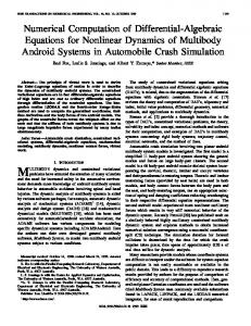
for the slope in the representation of the logarithm of the energy spectrum in terms of the logarithm of the wave number. According to Saffman [32], the dominant contribution in the energy spectrum comes from effects resulting from the discontinuities of vorticity. The value of the slope is then predicted to be of −4. However, the rough value which is obtained by numerical simulations is in general located between these two theoretical values. Besides Vassilicos and Hunt [37] pointed out that accumulating spirals above vortices make the flow more singular, so that the slope is attenuated, down to the value of −5/3. The creation of vorticity filaments leading to these accumulating spirals occurs during the vortices merging process [15]. This process transfers energy to larger scales, thus creating the inverse energy cascade. The overall energy spectrum is depicted in Figure 1. While several numerical simulations and experiments have shown results which agree in some relative way the theoretical predictions, few have really materialised the coexistence of both cascades [21], [6], [34], [35]. The experiment by Rutgers [31], using fast flowing soap films, remains one among such few realisations. Starting from Direct Numerical Simulations (DNS) of Navier-Stokes (NS) equations that reveal the coexistence of both slopes, the main goal of this paper is to point out the difficulties encountered when analysing the results. Indeed most of the methods are very sensitive to the various parameters and so the same method can lead to significantly different results according to the choice of the parameters. Therefore for each method we specify the adequate range of values to get relevant results. We consider the flow behind an array of cylinders in a channel with rows of small cylinders along the vertical edges of the channel (Figure 2). We will compare numerical methods (based on Fourier, wavelets and/or statistical models) that one can use to materialise (and then compute) energy spectra from numerical data (section 3). The section 4 will be devoted to decomposition/reconstruction methods based on the Karhunen-Loeve [24], [33] decomposition and cosine or wavelet packets. In the forthcoming part II such decomposition/reconstruction methods will be combined with a matching pursuit algorithm [26]. A complementary study of two-dimensional turbulence based on the velocity and the vorticity analysis will be addressed in another publication. Anyone who is interested in two-dimensional turbulence theory should refer to Lesieur [22], Frisch [10] or Tabeling [36] for a complete overview on the topic.
2
Description of the experiments and numerical results
The numerical simulation of a two-dimensional channel flow perturbed by arrays of cylinders, as on Figure 2 is performed. The length of the channel Ω is four times its width L ; the Reynolds number based on the diameter of the bigger
Comparison of numerical methods for the computation of energy spectra
3
3
10
2
10
−5/3
1
10
−3
0
10 E
−1
10
−2
10
−3
10
−4
10
0
10
1
10 k
2
k
10 injection
Figure 1: Theoretical spectrum cascades in 2D turbulence
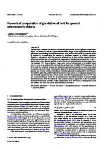
cylinders (equal to 0.1 × L) is Re = 50000. The experiment consists in solving numerically the NS/Brinkman model described below (1) in Ω = Ωs ∪ Ωf where Ωs (the ”obstacle” subset) is the union of the five horizontal disks together with 18 small disks (with diameter equal to 0.05 × L) and Ωf is the fluid domain as shown on Figure 2. The evolutions in time of the velocity (two components), of the vorticity and of the pressure have been recorded at a monitoring point located at (x 1 = 3L/8, x2 = 13L/16) sufficiently far away from the horizontal cylinders to take into account the developed turbulent events. These 1D temporal signals are then analysed and used to compute the energy spectra. Numerical results obtained through such DNS can be compared to those obtained in the experiments realised thanks to physical devices by Hamid Kellay in [7] : a soap film in a rectangular channel is disturbed by five big cylinders together with two rows of smaller cylinders. Let Ωf be the fluid domain, its boundary is defined by ∂Ω f = ∂Ωs ∪ΓD ∪ΓW ∪ΓN (see Figure 2). A non-homogeneous Poiseuille flow is imposed on the boundary ΓD as well as a no-slip boundary condition is imposed on the pieces of the boundary ΓW . The obstacles are taken into account by a penalisation procedure which consists to add a mass term in the equations which are now specified on the whole domain Ω as in [2]. Thus, we are looking for the solution of the
4
Ch.H. Bruneau, P. Fischer, Z. Peter, A. Yger
following initial boundary value problem : 1 U K div U
∂t U + (U · ∇)U − div σ(U, p) +
= 0 in ΩT = Ω × (0, T ) = 0 in ΩT
U (·, 0) = U0 in Ω U
= UD on ΓD × (0, T )
U = 0 on ΓW × (0, T ) 1 σ(U, p) · n + (U · n)− (U − U ref ) = σ(U ref , pref ) · n on ΓN 2 (1) where σ(U, p) is the stress tensor, U = (u, v) is the velocity vector, p is the pressure, U0 is the initial datum, UD the Poiseuille flow at the entrance section of the channel, U ref and pref a reference flow used to write non reflecting boundary conditions on the artificial exit section of the channel [8]. In this NS/Brinkman model, the scalar function K can be considered as the permeability of the porous medium. Numerical simulations are performed on rectangular meshes (1280×320 or 2560× 640 points) with a multi-grid approach. The two previous meshes correspond to grids 7 and 8 respectively. The time process lasts 40 units of non dimensional time with a step of 10−3 leading to 40000 output data for each temporal signal (pressure, components of the velocity and vorticity) at the monitoring point in Ωf . We see on Figure 3 that the velocity signals have roughly the same properties whereas the pressure and the vorticity signals exhibit huge picks corresponding to the convection of the coherent structures through the point position. In the following sections the Taylor hypothesis is used to convert time scales to length scales. This hypothesis has been thoroughly tested in such flows [4] and assumes that the flow structures are convected through the monitoring point without much deformation.
3 3.1
Energy spectrum computation The basic FFT method
The simplest way to visualise the energy spectrum corresponding to a given signal consists in computing the power spectrum of the first component of the velocity u. It is allowed to consider only the transverse velocity component since the flow perturbations are mainly isotropic and thus the power spectral densities of both velocity components are essentially the same. So they represent correctly the energy spectrum. A first na¨ıve attempt to perform such a computation has been done directly, applying the well known discrete Fourier transform to the whole velocity signal. Although this signal is not periodic, a windowed version
Comparison of numerical methods for the computation of energy spectra ΓD
5
x 1
Ωs ΓW
ΓW Ωf
ΓN x2
Figure 2: Computational domain
of the FFT method with functions such that Bartlett’s or Hanning’s is useless due to the large size of the signal. One can see immediately that graphical representations of the logarithms of the power spectra in terms of the logarithm of the wave number k (as represented on Figure 4 for the first component of the velocity signal) obtained that way provide a very noisy graph. Despite the thick aspect of the graph, it is possible to determine the slopes of both cascades through a first order least square approximation. Their value fits more or less with the theoretical values. One difficulty is the determination of the slope of the cascades as some parts of the spectrum have no physical or numerical meaning. Namely, the frequencies corresponding to a size bigger than the channel width and the frequencies corresponding to the unresolved scales. Let the unity be the channel width, then 1 . Due to that scaling, k ≈ 10 is the diameter of the horizontal cylinders is 10 the main frequency of injection. The diameter of the smaller cylinders in the 1 two vertical arrays is 20 which corresponds to an injection frequency of k ≈ 20. Moreover, the numerical simulation is performed on an uniform grid of mesh 1 1 size h = 320 or h = 640 . Assuming that for the representation of an oscillation generally we need 4 or 5 points, we expect to obtain significant scales between 1 the wave numbers corresponding to the half size of the channel k = 2 and k = 5h 1 or k = 4h . Thus it should be possible to determine correctly the two cascade slopes as following:
6
Ch.H. Bruneau, P. Fischer, Z. Peter, A. Yger
4
6
2
4
2
0 v
u −2
0
−4
−2
−6
p
0
10
20 time
30
−4
40
5
400
0
200
w
−5
−10
−15
0
10
20 time
30
40
0
10
20 time
30
40
0
−200
0
10
20 time
30
40
−400
Figure 3: Signals of the physical quantities at the monitoring point
Comparison of numerical methods for the computation of energy spectra
7
• for the inverse cascade (sl 1) between the frequencies k = 2 and k = 10 1 • for the enstrophy cascade (sl 2) between the frequencies 10 and k = 5h or 1 k = 4h . To confirm this assumption we perform numerous slopes computation on the en1 1 ergy spectrum obtained from simulation grids 7 (h = 320 ) and 8 (h = 640 ). On the Figure 5 the enstrophy cascade slopes (on the vertical axis) are determined always between the wave number k = 10 and the wave numbers represented in the horizontal axis. We can observe an almost constant behaviour in the vicinity of the wave number k = 65, while the first part of the curve is due to the influence of the injection scales and the last part is due to the dissipative 1 gives the same behaviour with tail. The same slopes computation for h = 640 an almost constant value around k = 130. This fact shows that by increasing the numerical simulation of the flow by a factor 2, we double the range of the enstrophy cascade. However, due to the thickness of the energy spectra, an accurate estimation of the slope is really hard to obtain. 3
10
−3.99 2
10
1
10
0
10 E
−1.86 −1
10
−2
10
−3
10
−4
10
0
10
1
10 k
2
10
Figure 4: Energy spectrum obtained for the first component of the velocity with Fourier method
3.2
The periodogram method
In order to overcome the difficulty arising in this na¨ıve approach, one can combine it with statistical ideas by computing the discrete Fourier transform of the digital signals [s(l), ..., s(l + p − 1)] for l = 1 : q : 40000 − p and averaging the graphic representations thus obtained for the logarithm of the energy spectrum. We still treat the first component of the velocity. The graphical representations obtained from the Bartlett windowed Fast Fourier Transform algorithm with the window size p = 2048 and the translation step q = 8 are plotted on Figure 6. Note that the thickness of the energy spectra is drastically attenuated, though the time-frequency information is of course lost since one uses a statistical process. Of course, when the size p of the window increases up to the size of the
8
Ch.H. Bruneau, P. Fischer, Z. Peter, A. Yger
−2.7
−2.7
−2.9
−2.9
−3.1
−3.1
−3.3
−3.3
−3.5 sl2
−3.5 sl2
−3.7
−3.7
−3.9
−3.9
−4.1
−4.1
−4.3
−4.3
−4.5
−4.5
−4.7
20
40
60 k
80
−4.7
100
20
40
60
80
100
120
140
160
180
200
k
(a) simulation on grid 7
(b) simulation on grid 8
Figure 5: Determination of the upper bound to evaluate the enstrophy cascade slope signal, one recovers the thick energy spectra plotted on Figure 4. The Figure 7 shows the evolution of the estimated slopes respect to the size p (between 10 3 and the extreme value 39 × 103 ) of the window when q is kept equal to 10. The slope within the inverse cascade range remains essentially located around −1.8, while the slope within the enstrophy cascade range takes values around −4 like in the previous subsection. Let us point out to the reader that when the size p of the window is small it is necessary to use windowed Fast Fourier Transform to reduce the effect of the side lobs that introduce high frequencies and so modify the slope in the high frequency part of the spectrum. This is illustrated on Figure 8 where the slopes of the spectra obtained without windowing are about the same than those of Figure 7 except for small sizes p ≤ 10000 in the enstrophy cascade. 3
10
−1.78 −4.06
2
10
1
10
0
10 E
−1
10
−2
10
−3
10
−4
10
0
10
1
10 k
2
10
Figure 6: Energy spectrum obtained by the periodogram method with p = 2048 and q = 8 for the first component of the velocity
9
Comparison of numerical methods for the computation of energy spectra
−1
−3.2
−1.2
−3.4
−1.4
−3.6
sl1
sl2 −1.6
−3.8
−1.8
−4
−2
0
10000
20000 window size
30000
−4.2
40000
0
(a) inverse cascade
10000
20000 window size
30000
40000
(b) enstrophy cascade
Figure 7: Evolution of the slopes in terms of the size of the window with the Bartlett windowed periodogram method
−1
−3.2
−1.2
−3.4
−1.4
−3.6
sl1
sl2 −1.6
−3.8
−1.8
−4
−2
0
10000
20000 window size
30000
(a) inverse cascade
40000
−4.2
0
10000
20000 window size
30000
40000
(b) enstrophy cascade
Figure 8: Evolution of the slopes in terms of the size of the window with the periodogram method
10
3.3
Ch.H. Bruneau, P. Fischer, Z. Peter, A. Yger
The correlation method
One can determine the power spectral density of a signal as being the Fourier transform of the auto-covariance function. By the indirect (or the BlackmanTukey) method, in a first stage one estimates the auto-covariance function and then, by taking the Bartlett windowed Fourier transform of this function one calculates the power spectral density. Let be x n , (n = 0, 1, 2..., N −1) the studied signal containing N samples. A biased estimate of the auto-covariance function is given by: 1 e R(Q) = N
N −Q−1 X
xn+Q xn
with
Q = 0, 1, . . . , N − 1
(2)
n=0
The values of this function for the negative arguments can be deduced starting from the estimates obtained for the positive arguments by the relation: e e R(−Q) = R(Q).
(3)
In our case N = 40000 and we will calculate the power spectral density of the signal using M ≤ N correlation coefficients. The results obtained for the energy spectrum, still for the first component of the velocity is displayed on Figure 9. When M is small the slopes are underestimated with an error up to 14% whereas the results are coherent with those obtained in the previous subsections for M ≥ 10000. On the Figure 10 we represent on the vertical axis the various values of the slopes for the variation of the correlation coefficients in the autocovariance method. One can see the decreasing behaviour especially on the level of enstrophy cascade while the slope of the inverse cascade remains roughly the same one except for M = 1000. These graphs can justify the choice of the needed correlation coefficients in the calculation of the slopes of the power spectrum. An insufficient number of coefficients can yield more than 10% of error. However in this computation the choice of the windowing function is very important as the same study with Hanning function gives much better results, especially for the direct cascade. Like in the periodogram, we can calculate the power spectral densities on some smaller windows and, taking the mean, obtain the estimated energy spectra (Welch method with no overlaps). Let x n , (n = 0, 1, 2..., N − 1) be a digital signal (interpreted as a stationary process) with length N , we choose a window size p. Let us set the number of parameters M = E[p/2], an unbiased estimate for the auto covariance function is given by : h p−1−k i X 1 xn×p+l+k xn×p+l , k ∈ {0, ..., M − 1} → averagen p l=0
where the averaging process is taken over values of n between 0 and E[N/p]. On the Figure 11 are presented the results obtained with 20 windows of length
Comparison of numerical methods for the computation of energy spectra
11
2000. For each such a window we determine 1000 correlation coefficients and then the estimation of the energy spectra is obtained by taking the mean of the power spectral densities. Here again the results are not correct as the size of the window is too small. Indeed, the estimated slopes obtained when one interprets energy spectra as power spectral densities of stationary processes depend on the value of the size p. The Figure 12, shows the evolution of the two estimated slopes in terms of the value of such a size p when p increases from 1000 up to 20000. Once again a size at least p ≥ 5000 is required to get reliable results. This is coherent with the fact that the validity of the correlation method lies on the assumption that the signal remains stationary on windows of size p. Indeed we can check on the correlation matrix given in the Figure 13 that the stationary assumption is much more fulfilled for p = 20000 than for p = 1000. In conclusion there is a significant variation of the slopes with respect to the size p of the window which is used to compute the auto correlation. Relatively large values of p better verify the stationary assumption and thus the resulting slope is in very good accordance with the slopes obtained with the periodogram method in subsection 3.2. 3
10
−3.87 2
10
1
10
−1.72
0
10 E
−1
10
−2
10
−3
10
−4
10
0
10
1
10 k
2
10
Figure 9: Energy spectrum obtained by the correlation method
3.4
The method based on the auto regressive model
Let us consider again the digital real signal (x n )n , n = 0, ..., N − 1, corresponding for example to the measurements of the first component of the velocity, as a discrete stationary process. The search for an optimal auto regressive model with an a priori prescribed number of parameters m < N ) consists in the de-
12
Ch.H. Bruneau, P. Fischer, Z. Peter, A. Yger
−1
−3.2
−1.2
−3.4
−1.4
−3.6
sl1
sl2 −1.6
−3.8
−1.8
−4
−2
0
5000
10000 M
15000
−4.2
20000
(a) inverse cascade
0
5000
10000 M
15000
20000
(b) enstrophy cascade
Figure 10: Slope estimates computed with the correlation method in terms of M
3
10
−1.45 2
10
−3.28 1
10
0
10 E
−1
10
−2
10
−3
10
−4
10
0
10
1
10 k
2
10
Figure 11: Cascades slopes computed with the correlation method using Welch method with 20 non overlapping windows of size p = 2000
13
Comparison of numerical methods for the computation of energy spectra
−1
−3.2
−1.2
−3.4
−1.4
−3.6
sl1
sl2 −1.6
−3.8
−1.8
−4
−2
0
5000
10000 window size
15000
−4.2
20000
(a) inverse cascade
0
5000
10000 window size
15000
20000
(b) enstrophy cascade
Figure 12: Slope estimates computed with the Welch correlation method in terms of the window size
0
0
200
4000
400
8000
600
12000
800
16000
1000
0
200
400
600
800
(a) with a 1000 points window
1000
20000
0
4000
8000
12000
16000
20000
(b) with a 20000 points window
Figure 13: The correlation matrices for different time windows calculated for the first component of the velocity
14
Ch.H. Bruneau, P. Fischer, Z. Peter, A. Yger
termination of estimators µ, α1 ,...,αm such that S(µ, α1 , ..., αm ) :=
N X
zn2
n=m+1
=
N X
h
(xn − µ) − α1 (xn−1 − µ) − · · · − αm (xn−m − µ)
i2
n=m+1
is minimal. In order to seek for such estimators, the use of the least squares criterion takes its justification from the a priori assumption that the residual process zn := (xn − µ) −
m X
αl (xn−l − µ) , n = m, ..., N − 1 ,
(4)
l=1
is Gaussian with mean value 0 and variance σ z2 which means that µ corresponds essentially to the mean value of the digital process. Optimal values α c1 , ..., αc m for the coefficients α1 , ..., αm are then computed through the Yule-Walker method [30], [14], and the corresponding numerical model for the power spectral density of the stationary process realised by the digital signal (x n )n is ω ∈ [0, π] → Sxx (ω) =
s2z 2 , |1 − α c1 exp(−iω) − ... − αc m exp(−imω)|
(5)
where s2z denotes an unbiased estimate for the residual variance σ z2 , obtained when m