Comparison of two different identification algorithms
nonlinear
state-space
Johan Paduart, Johan Schoukens, Kris Smolders, Jan Swevers Vrije Universiteit Brussel, dep. ELEC, Pleinlaan 2, 1050 Brussels, Belgium e-mail:
[email protected]
Abstract In this paper, a comparison between two models for nonlinear systems is made. Both models have a state space nature, but there are some differences in the identification approach and the model structure. The first model that we will discuss is a discrete time model that uses input-output data for the identification. The second model uses explicit measurements of the states of the system and some physical insight to model the relationship between the states. The similarities and differences between the two models are discussed, and their performance is compared utilizing data from an experimental setup.
1
Introduction
A choice can be made between numerous (black box) model structures when modelling a nonlinear system (e.g. Wiener/Hammerstein/Wiener-Hammerstein models, LS-SVM,...) but most of them are dedicated to single input single output (SISO) systems. Models using a state space approach, like Local Linear Models, LPV’s, bilinear systems [1] have the advantage that the identification methods can easily be extended to the multivariable case. In this paper we will compare two nonlinear state space models. The structure of this paper is as follows: First, we will explain the concept of Best Linear Approximation (BLA), which is used in the (common) first step of the two methods described in this paper. Then, both nonlinear model structures and identification methods will be explained. Finally, the performance of the two models is compared using experimental data.
2
Best Linear Approximation
When building a nonlinear model for a system, it is always a good idea to start from a linear framework. As it happens, most of the dynamic behaviour of a Device Under Test (DUT) can be described by a linear model, for which numerous identification techniques are available. By adding nonlinear features in the second phase of the identification procedure, the model performance can be enhanced. That is why both identification methods that are the subject of this paper will begin by estimating a linear model and extend it in order to grasp the nonlinear behaviour. The following question then arises: how to obtain a good linear model for a nonlinear system? We will do this by determining the Best Linear Approximation (BLA) of the system. The BLA is the best linear (nonparametric) model in least squares sense for a nonlinear system, for a given class of input signals [2]. Restricting ourselves to the class of Gaussian signals, we can make use of random phase multisines to determine the BLA. A multisine signal is a periodic signal, defined as the sum of a number of harmonically related sines, with a user selected amplitude. The phase is chosen uniformly distributed over [ 0, 2π) . Several advantages pop up when utilizing these excitation signals. By putting the even and some of the odd frequency lines to zero, the level of even and odd nonlinearities can be inspected by looking at the unexcited lines, or so called detection lines, at the output. The excited lines are used to compute the Frequency Response Function (FRF) of the system under test. A number of phase realizations of the multisines can be applied to the DUT to determine the FRF for each of these experiments. By averaging the FRF’s over the experiments, a nonparametric estimate of the BLA can be obtained [2]. Then, 2777
2778
P ROCEEDINGS OF ISMA2006
the approximate linear model for the nonlinear DUT can be estimated based on the averaged FRF data.
3 3.1
Nonlinear Polynomial State Space Model Model Structure
The first nonlinear model that we will discuss is based on the linear, discrete time state space equations. x ( k + 1 ) = Ax ( k ) + Bu ( k )
(1)
y ( k ) = Cx ( k ) + Du ( k )
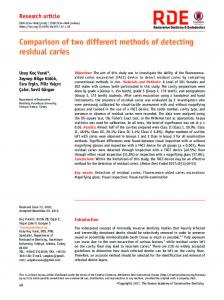
In equation (1), x ( k ) is the ( n × 1 ) state vector, u ( k ) the ( m × 1 ) input vector and y ( k ) the ( p × 1 ) output vector at time instant k . A , B , C , and D are the linear system matrices. A graphical representation of this model is given in Figure 1.
u
B
z
–1
C
y
A D Figure 1: Graphical representation discrete time state equations In order to model nonlinear systems, the linear model is extended with multivariable nonlinear functions f and g : x ( k + 1 ) = Ax ( k ) + Bu ( k ) + f ( x ( k ), u ( k ) )
(2)
y ( k ) = Cx ( k ) + Du ( k ) + g ( u ( k ) )
u
B
z
–1
C
y
A D
Figure 2: Graphical representation of extended nonlinear state equation The nonlinear functions f and g can take an arbitrary form. We will use a multivariable polynomial expansion and define the nonlinear functions as a product of a coefficient matrix and a vector of monomials (the time index k is omitted for notational simplicity).
N ON - LINEARITIES : IDENTIFICATION AND MODELLING
2
f ( [ x ;u ] ) = F x ×
2
2779
2
x1
u1
u1
x1 x 2
u1 u 2
u1u2
Fx ∈ ℜ
…
Fu ∈ ℜ
… r–1 xn – 1 x n r
xn
+ Fu ×
g ( u ) = Gu ×
… s–1 um – 1 um
t–1 um – 1 um
s
t
um
n × L ( n, r )
n × L ( m, s )
Gu ∈ ℜ
(3)
p × L ( m, t )
um
The vector of monomials is composed of all possible combinations of input components until a certain degree. If there are n components of the vector of which the monomials are formed, and the degree of nonlinearity is r , the resulting monomial vector has length L ( n, r ) : r
L ( n, r ) =
∑ ⎛⎝
n + i – 1⎞ ⎠ i
(4)
i=2
In other words, there is a combinatorial growth in the number of nonlinear parameters as the system order n or input number m increases. To circumvent a huge number of parameters, a limited set of monomials can be selected when high order models are fitted, for instance only the “pure” powers i.e., without cross products between the components.
3.2
Identification
The identification problem associated with the model described in the previous section is nonlinear in the parameters. Therefore, a nonlinear optimization has to be performed to obtain optimal parameter values. For an optimization problem, it is advantageous to utilize good starting values. That is why the identification process is split up in two parts: one part to obtain decent starting values and the second part which consists of solving a nonlinear optimization problem minimizing the quadratic distance between the modelled and measured output. 3.2.1. Starting Values First we will determine the BLA of the system, as described in section 2. From this nonparametric model, a linear parametric state space model is estimated using Frequency Domain Subspace Identification ([3],[4]). This results in a linear model described by x ( k + 1 ) = A BLA x ( k ) + B BLA u ( k ) y ( k ) = CBLA x ( k ) + D BLA u ( k )
(5)
The system matrices of this linear model can be used as starting values for parameters A , B , C and D of the nonlinear model described in equation (2). The initial values of parameters F x , F u and G u from (3) are set to zero. This way, the nonlinear model will perform at least as good as the best linear model.
2780
P ROCEEDINGS OF ISMA2006
3.2.2. Nonlinear optimization The formulation of the optimization problem is as follows: we use a Weighted Least Squares approach, formulated in the time domain since this is the most appropriate domain to compute the nonlinear terms. The cost function to minimize is defined as p
V WLS =
N
( yi, meas ( k ) – y i, model ( k ) ) 2 ∑ ∑ -----------------------------------------------------------2 ( k ) σ y i = 1k = 1
(6)
2
The variances σ y ( k ) can be obtained from the measured data, since we collected several periods of the periodic signals that we used to excite the system. The cost function can be minimized with a Levenberg-Marquardt (L.M.) algorithm, for which the Jacobian J (the matrix of derivatives of the model output to the parameters) is needed. To compute the Jacobian, it is necessary to obtain initial values for the states. This can be seen in the following example, where we compute the Jacobian for the elements of the system matrix A JA ( k ) = ij
∂ ∂ y(k) = C x(k) ∂ A ij ∂ A ij
(7)
where element ( i, j ) of A is denoted as A ij . If we define ∂ x(k) ∂ A ij
(8)
∂ ∂ A ⋅ x ( k – 1 ) + A ⋅ Jx A ( k – 1 ) + F x ⋅ w(k – 1 ) ∂ A ij ij ∂ A ij
(9)
Jx A ( k ) = ij
then it follows that: Jx A ( k ) = ij
where w ( k ) is the vector of monomials in x ( k ) . The expressions for JB ( k ) , JC ( k ) , J D ( k ) and J N L ( k ) are ij ij ij ij computed similarly. From these expressions, the following can be concluded: The calculation of the Jacobian has to be performed recursively: to calculate Jx A ( k ) , Jx A ( k – 1 ) is ij ij needed. • One also needs estimates of the states x ( k – 1 ) . To obtain these, the calculated states from the previous iteration in the Levenberg-Marquardt loop are used. •
A last issue that needs to be addressed before we can handle the optimization, is the rank deficiency of the Jacobian J , which is present due to the non-uniqueness of the state space representation. A similarity transformation –1 x˜ ( k ) = T x ( k ) leaves the input-output behaviour of the state space model unaffected. As a consequence, the 2 Jacobian J will not be of full rank. This rank deficiency of n can be taken care of by using a truncated Singular Value Decomposition when computing the pseudo inverse of J , [5]. When the Jacobian is available, the Levenberg-Marquardt algorithm can be started. The used stop criterion consists –6 of a minimal relative decrease of the cost function (e.g. 10 ). After reaching this criterion, all the fitted models (i.e., obtained after each successful L.M. step) are cross-validated on a second data set. The model with the lowest (weighted) error in the validation set is selected. This way, overfitting on the estimation set is avoided.
N ON - LINEARITIES : IDENTIFICATION AND MODELLING
4 4.1
2781
Nonlinear State Space Model with a Feature Space Transformation Model Structure
The continuous time model structure proposed here is · x = Ax + Bu + Wz ( x )
(10)
y = Cx + Du + Tz ( x )
Vector z with dimensions s × n is defined as a sigmoidal function of the states x 1 1 z j ( x ) = ---------------------------------- – -----------------–( V j x + gj ) –gj 1+e 1+e
(11)
with V1 V = … Vs
V∈ℜ
s×n
g1 and
g = … gs
g∈ℜ
s
(12)
The advantage of these sigmoidal functions, which are very common in the neural network theory, is the “nice” behaviour they show when extrapolating. Polynomial models tend to explode when they are used outside the estimation range. The disadvantage is that more features thus parameters might be needed to describe (static) nonlinear behaviour, depending on the type of nonlinearity.
4.2
Identification
In this approach it is assumed that the states x can be measured. Since periodic signals were used to excite the system, the derivatives x· don’t need to be measured since they can be obtained correctly in a numerical way. An iterative scheme is then used to determine the model parameters. First, the BLA is determined between { x· , y } and { x, u } . The residuals of this linear model are then used to estimate the sigmoidal features. The linear model is then refined, and so on. The advantage of this grey box approach is that a priori information about the system can be included. However, the drawback is the need for more sensors. Furthermore, not all states can always be measured in practical situations, or be determined unambiguously. More details about the identification procedure can be found in [6].
5
Experimental Results
Both models were used to model the behaviour of the quarter car set-up located at the department of PMA, KULeuven [6]. This physical set-up is a scale model of a suspension of a car based on masses, springs and a nonlinear semi-active damper. The road displacement of the wheel is considered as input, the force measured over the damper as the output of the system. Two odd multisines, consisting of 10 periods were applied to use for estimation purposes. The linear models were fitted on the BLA computed from the two multisines while the nonlinear models were fitted on the first multisine and cross validated with the second multisine. A filtered noise sequence with increasing amplitude over time was applied to the system for validation purposes.
2782
P ROCEEDINGS OF ISMA2006
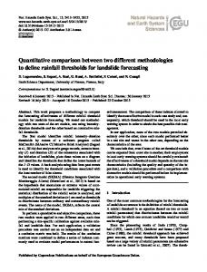
For the polynomial nonlinear model, a 5th order linear model was estimated. The monomial vectors associated with F x were composed of powers [2 3 4 5]; G u and F u were set to zero. Without any precautions, this model would need 246 × 5 parameters for the nonlinear state contributions only. By using a diagonal type of structure, r r without cross products i.e., only monomials of type x i ( k ) contributing to x i ( k + 1 ) , the number of nonlinear parameters is reduced to 4 × 5 = 20 . Together with the linear parameters this results in a total of 56 parameters. The second nonlinear model starts from a 6th order linear model, and 18 features, resulting in a total of 133 parameters [6]. The validation results are shown in Table 1, by means of the Root Mean Square (RMS) values of the error signals of the different models. Since the amplitude of the noise sequence exceeds the amplitude of the multisines used during estimation, a distinction is made between the normal and extrapolating behaviour of the models. This can be done by comparing the (piecewise) RMS level of the noise input sequence with the RMS level of the estimation input data set (Figure 3, (a)). The first row in Table 1 indicates the RMS levels of the model errors for the whole dataset i.e., including the region where the extrapolation takes place. The bottom row only takes into account the normal, non-extrapolating behaviour, which is the fairest way to evaluate the model performances. In general, it is not a good idea to use nonlinear models outside their estimation region, because the nonlinear characteristics must have been “seen” in order to simulate the system’s behaviour accurately. From these results we can conclude that the polynomial nonlinear model performs better than the model utilizing the sigmoidal features. This is probably caused by the fact that prior knowledge was included in the construction of the second model [6], which was not completely correct. The black box model has more flexibility to capture this behaviour. RMS Output Signal
Polynomial Approach
Sigmoidal Features Approach
Linear Model
Nonlinear Model
Linear Model
Nonlinear Model
Validation
0.242
0.139
0.052
0.166
0.089
Validation without extrapolation
0.212
0.124
0.046
0.156
0.080
Table 1: Validation Results: RMS Values Model Error Signals
N ON - LINEARITIES : IDENTIFICATION AND MODELLING
2783
(a) Determination of Extrapolation 0.3 Extrapolation Input Signal RMS Validation RMS Estimation
Input Signal
0.2 0.1 0 −0.1 −0.2 0
40
60
80 100 Time [s] (b) Nonlinear Polynomial State Space Model
120
40
60
120
40
60
Extrapolation Measured Lin. Model Error NL. Model Error
0.5 Output Signal
20
0
−0.5 0
80 100 Time [s] (c) Nonlinear State Space Model with a Feature Space Transformation
Extrapolation Measured Lin. Model Error NL. Model Error
0.5 Output Signal
20
0
−0.5 0
20
80
100
120
Time [s]
Figure 3: Validation Results
6
Conclusion
In this paper we have compared two nonlinear state space models. The advantage of the nonlinear polynomial model is that it does not need any prior knowledge about the system to model its input-output behaviour. At the same time, this forms the drawback of this approach: the resulting model cannot be used to interpret the system’s behaviour physically. Also sometimes it can be interesting to add prior knowledge to the model, in that case the second approach is more suitable. In general, less parameters are then necessary; thus a lower variance on the parameter values is obtained. However systematic errors might be introduced if wrong assumptions are made. We can conclude that the user, before estimating a nonlinear model, should decide what he or she wishes to achieve. In a simulation or MPC environment, a blackbox model is more suitable. When physical insight is needed, the grey box approach is more appropriate, but in that case the black box approach can still be used to verify if the physical
2784
P ROCEEDINGS OF ISMA2006
model captured the full behaviour.
Acknowledgements This work was supported by the FWO-Vlaanderen, the Flemish community (Concerted action ILiNoS), and the Belgian government (IUAP-V/22).
References [1] Verdult, V. (2002). Nonlinear System Identification - A State Space Approach. Twente University Press [2] Schoukens J., R. Pintelon, T. Dobrowiecki, and Y. Rolain (2005). Identification of linear systems with nonlinear distortions. Automatica, Vol. 41, No. 2, pp. 491-504 [3] McKelvey, T., H. Akçay and L. Ljung, (1996). Subspace-based multivariable system identification from frequency response data. IEEE Transactions on Automatic Control, 41(7), pp. 960-979. [4] Pintelon, R. (2002). Frequency-domain subspace system identification using non-parametric noise models. Automatica, Vol. 38, pp. 1295-1311. [5] Golub, G. H., C. F. Van Loan (1996). Matrix Computations - Third Edition. The John Hopkins University Press, London. [6] Smolders, K., M. Witters, J. Swevers, P. Sas (2006). Identification of a Nonlinear State Space Model for Control using a Feature Space Transformation. Proceedings of the ISMA2006 Conference.