Comparisons of Three Kalman Filter Tracking Algorithms in Sensor Network Yifeng Zhu and Ali Shareef∗ Department of Electrical and Computer Engineering University of Maine, Orono, ME 04469, USA Email:
[email protected] and Ali
[email protected] Abstract
2 2D Tracking Algorithms
This paper compares extended Kalman filters with the P, PV and PVA dynamics models for object tracking in wireless network. Experiments shows that PVA achieves the best and P performs the worst in most cases. In addition, increasing the number of pivots can slightly improve the tracking accuracy.
The problem of tracking a moving device in sensor network is summarized as follows: Given N fixed pivots at known positions and distance measurements to these pivots, find the position where the target object is located. As shown in Fig. 1, the challenge lies in that distance measurements are inaccurate and also the speed and acceleration cannot be directly measured. We use Extended Kalman Filter (EKF) [3] to solve the tracking problem in this paper. Based on the amount of internal states that the target estimates, there are three dynamical EKF models in tracking.
1 Introduction Tracking is a fundamental system-level issue in wireless sensor networks since it can provide a crucial context for measurements taken in an environment [1]. In many applications, such as environmental monitoring or intrusion detection, tracking the location of an event or object is almost as important as the detection of the event or the measurement of the object. Tracking is also of great importance in applications where measurements are collected through the cooperation of many fixed cheap wireless communication sensors and multiple expensive mobile sensors. A lot of research has been conducted to tackle this problem of tracking [2].
1. Position Model(P Model): The state vector includes its position only. 2. Position-Velocity Model(PV Model): The state vector includes its position and velocity. 3. Position-Velocity-Acceleration Model(PVA Model): The state vector includes its position, velocity, and acceleration. The following takes the PV model with 3 pivots as an example to illustrates our tracking algorithms. Let X = [x, y, x, ˙ y] ˙ T and D = [d1 , d1 , d3]T where di = p 2 (x − xi ) + (y − yi )2 and (xi , yi ) is the location of Pivot i. The State equations is given as follows.
trajectory
y x
Pivot 1
·
D1 D2 Pivot 2
Xk+1
Target (x, y, v, a)
=
AXk + B
ux k uy k
¸ ˜k +X
(1)
1 2 0 1 0 T 0 2T 1 2 0 1 0 T 0 2T , where A = 0 0 1 0 , B = T 0 0 0 0 1 0 T ˜ k is (ux , uy ) are control forces in the x and y axis, and X system process white noise. The Output equations can be written as
D3 Pivot 3
Figure 1. The Tracking Curve of PV model. ∗ This work was supported by National Science Foundation grant 0538457 and an UMaine Startup Fund.
˜k Dk = Dk + D 1
(2)
˜ k is measurement white noises. The output equawhere D tions can be linearized at position k as follows.
6
12
x 10
100
PV
1
=
∂x ∂d2 ∂x ∂d3 ∂x
1
∂y ∂d2 ∂y ∂d3 ∂y
0 0 ˜k 0 0 Xk + D 0 0
(3)
6 Moving Trajectory PVA Tracking 4
80
Cumulative Distribution Function
˜k = HXk + D ∂d ∂d
Y
8
PV Tracking P Tracking
60 50 40 30 20
(4)
10 0 −4
−3
−2
−1
0
1
0 0
2
X
=
p
∂di ∂y
=
p
x − xi (x − xi )2 + (y − yi )2 y − yi (x − xi )2 + (y − yi )2
1
2
3
4
6
5
6
7
Error
x 10
Figure 2. Output of tracking algorithms
where ∂di ∂x
P
70
2
8
9
10 4
x 10
Figure 3. Accuracy Comparison of P, PV, PVA
(5)
PVA Tracking 100
(6)
for i = 1, 2, 3. The following steps describe equations that need to be evaluated on-line for an EKF. Algorithm 1 EKF Tracking ˆ − = AX ˆ k−1 + BUk and calculate D− 1: Project the state ahead: X k k − ˆ based on Xk 2: Project the error covariance ahead: Pk− = APk−1 AT + W Qk−1 W T ; 3: Compute the Kalman gain: Kk = Pk− HkT (Hk Pk− H T + Vk Rk VkT )−1 ; 4: Update estimation with measurements: ˆk = X ˆ − + Kk (Dk − D− ); X k k 5: Update the error covariance: − Pk = (I − Kk Hk )Pk ; 6: Repeat and go to Step 1.
where W and V are the Jacobian matrix of partial derivatives of state and output functions with respect to the process noise and measurement noise, respectively. P , R and Q are the covariance matrix of the error in the state estimate, measurement noise, and process noise, respectively.
3 Performance Comparison We have implemented EKF P, PV, and PVA tracking algorithms and performed experiments extensively. Due to space limitation, we only present one group of experiments. The parameters of different algorithms are kept the same as much as possible in order to provide a fair comparison. Fig. 2 shows estimated moving curves when three pivots are deployed and Fig. 3 compares the accuracy of these three algorithms in this case. In Fig. 2, the output of PVA almost overlaps with the moving trajectory of the target object. As shown in Fig. 3, PVA is the best tracking model while P is the worst one in these experiments. In fact, in other experiments, PVA is almost consistently better than PV and P, while in a very few cases PV achieves the best.
3 pivots 50
Cumulative Distribution Function
Dk
PVA
90 10
0
5 pivots
0
500
1000
1500
2000
2500
Error
PV Tracking
100 3 pivots
50
5 pivots 0
0
2
4
6 Error
8
10
12 4
x 10
P Tracking
100
3 pivots
50
5 pivots 0
0
0.5
1
1.5
2 Error
2.5
3
3.5
4 6
x 10
Figure 4. Impact of the pivot number.
We also evaluate the impact of the number of pivots on tracking accuracy. Fig. 4 shows that the performance when five pivots are deployed is better than the experiments with only three pivots. But the performance with only four pivots, not shown in the paper, is almost the same as that of five pivots.
4 Conclusions and Future Work This paper compares extended Kalman filters with the P, PV and PVA dynamics models for object tracking in sensor network. We are porting our implementation into wireless sensors.
References [1] L. Hu and D. Evans, “Localization for mobile sensor networks,” in roceedings of the 10th annual international conference on Mobile computing and networking, 2004, pp. 45–57. [2] AdamA. Smith, H. Balakrishnan, M. Goraczko, and N. Priyantha, “Tracking moving devices with the cricket location system,” in Proceedings of the 2nd international conference on Mobile systems, applications, and services, 2004, pp. 190–202. [3] Ian R. Petersen, Robust Kalman Filtering for Signals and Systems with Large Uncertainties, Birkhauser Boston, 1999.