IEEE TRANSACTIONS ON VEHICULAR TECHNOLOGY, VOL. 51, NO. 3, MAY 2002
577
Compensation of Axle-Generator Errors Due to Wheel Slip and Slide Samer S. Saab, Senior Member, IEEE, George E. Nasr, and Elie A. Badr
Abstract—Significant errors of train axle generators (tachometers) are due to wheel slip and slide. In this paper, an algorithm is designed to compensate for these errors. The algorithm identifies the wheel slip and slide by examining the variation of the processed vehicle longitudinal acceleration. Whenever wheel slip/slide is identified, then the vehicle speed is adjusted if a certain condition is met. The adjustment is a simple linear interpolation between the two speed values recorded before and after wheel slip/slide detection. In addition, a speed and acceleration observer using a Kalman filter is implemented. Experimental results using three different axle encoders aboard a freight train are provided to illustrate the performance of the proposed algorithm. Index Terms—Axle generator, Kalman filtering, train positioning, wheel slip and slide.
I. INTRODUCTION
I
N recent times, the Federal Railway Administration (FRA) and numerous railway companies are considering to disregard the fixed block system or track circuits and use another system essentially to improve safety [1] and deliver significant operating benefits. This system must minimize collision between trains, unauthorized train encroachment of authority limits, and locomotive overspeed operation. In addition, accurate position stopping, arrival time, and optimization control of the trains to move a maximum number of passengers or freight are also desired. Many companies such as Harmon, Union Switch & Signal, Rockwell, GE–Harris Railway Electronics, etc., proposed different computer and radio-aided train control systems [2], [3]. These systems control the train by radio and make the train itself estimate its own position. Most of the proposed train positioning systems make use of axle generator(s) or tachometer(s) [2], [4]–[8]. Doppler radar sensors are also considered for speed measurement [9], however, the problem with Doppler radar is the fundamental variability in the received signal using the track as a target. The employment of axle generators is due to the low cost, availability, reliability, and accuracy associated with such sensors. Unfortunately, due to the nonsteerable truck design associated with rail vehicles and poor adhesion, the wheel slips and slides. Most of the wheel slips and slides occur whenever the vehicle is going through a curve, accelerating, decelerating, climbing, or navigating on a wet track. Consequently, errors Manuscript received September, 1998; revised September, 2001. This work was supported by the University Research Council at the Lebanese American University. The authors are with Lebanese American University, 48328 Byblos, Lebanon (e-mail:
[email protected]). Publisher Item Identifier S 0018-9545(02)04950-2.
in speed and distance traveled measurements are produced. Several traction controller techniques are considered to minimize wheel slip/slide phenomenon (the reader is referred to [10]–[13]). However, complete control over wheel slip and slide has not been claimed yet. Recently [14], the design of a correlation system for noncontact speed measurement of rail vehicles is proposed. The correlator, used for deriving the speed, employs eddy current sensors. To the best of the authors’ knowledge, this paper presents the first attempt to formulate a computational algorithm for detecting wheel slip and slide using an axle generator. In this paper, a novel algorithm is proposed which compensates the distance traveled errors due to wheel slip and slide using an axle generator. The compensation is accomplished right after the wheel stops from slipping or sliding for a short time interval. First, a steady-state Kalman filter is implemented to observe the vehicle longitudinal speed and acceleration. Then, identification of wheel slip and/or slide is achieved by examining the variation of the processed vehicle acceleration. Finally, whenever wheel slip/slide is identified, then the vehicle speed during the identified slip/slide mode interval is adjusted if a certain necessary condition is met. The adjustment is a simple linear interpolation between the two speed values recorded before and after wheel slip/slide detection. Moreover, experimental results are included to illustrate the performance of the proposed algorithm. In Section II, we present an axle-generator error model, formulate some characteristics of wheel slip and slide development, and present the proposed algorithm. In Section II, we also show a major drawback whenever implementing an acceleration adjustment algorithm. In Section III, we describe the experiment, show the design of the vehicle speed and acceleration observer, and present the results. Finally, we conclude in Section IV.
II. PROPOSED ALGORITHM FOR WHEEL SLIP AND SLIDE COMPENSATION A. Preliminary The basic idea is to compensate for the distance traveled errors, which are due to wheel slips and slides whenever an axle generator (or tachometer) is employed as a distance traveled measurement sensor. In this paper, wheel slip is thought of as a wheel rotating faster than a nominal wheel. A nominal wheel is a fictitious and an “ideal” wheel, which does not slip nor slide. Conversely, wheel slide is a wheel rotating slower than
0018-9545/02$17.00 © 2002 IEEE
578
IEEE TRANSACTIONS ON VEHICULAR TECHNOLOGY, VOL. 51, NO. 3, MAY 2002
a nominal wheel. Let and be the radius and angular velocity of a nominal wheel. Consequently, the true linear speed . The processed speed measurement is given by (1) where the error
may be modeled as (2)
and are errors associated with the represents calibration wheel slip and slide, respectively, error due to errors in measurement of the corresponding wheel radius, wheel wear, and/or wheel circumference not being a perfect circle. Note that may be modeled as slowly time-varying depicts errors due to tachometer quantization. parameter. The processed angular velocity is given by (3) where (4) With frequent wheel calibration and employment of appropriate tachometer, the errors due to calibration and quantization become much smaller than the errors due to slip and slide, where they may be neglected. Automatic wheel calibration may be achieved by the use of a global positioning system (GPS) receiver. In particular, within particular open regions (where the signals of the GPS satellites are not obstructed, the track is straight and flat, and the vehicle is moving at a constant speed), the errors due to slip and slide can be neglected. Furthermore, if the wheel calibration is “remarkably” off, then quantization errors can also be neglected. For example, if this particular track is 1000 m long and the wheel circumference is 3 m and, assuming that the errors due to GPS measurements are about 15 m, then . If a differential GPS (DGPS) it can be shown that receiver is employed, then we may assume that DGPS measure. ments errors are about 1 m, consequently, Note that if we assume that the wheel slips as much as it slides and we neglect the errors due to calibration and quantization, then, in the limit, the distance traveled is given by
Therefore, in the long run, the combined contribution of the errors due to slip and slide in the overall vehicle distance traveled tends to be zero. Unfortunately, this is not the case. In fact, considering normal operation, the wheel slides more
than it slips [15]. Consequently, one may speculate that . In order to decrease the magnitude of errors due to slip and slide, one should examine the slip and slide characteristics during normal operations. One important point is that the wheel cannot slip and slide simultaneously. Thus, we have three ; either cases for a sufficiently small time period and and , and . Another major attribute is or that while a wheel is slipping or sliding it is always striving to and ). go back to its nominal mode ( Therefore, one may state the following. Postulate 1: Assuming navigation over a sufficiently long , where track segment, there exist time intervals such that the vehicle speed error depends only on . the calibration and/or quantization errors Also, when traveling in a straight track at a constant speed, the occurrences of wheel slip and slide are expected to be less than whenever the vehicle is accelerating, decelerating, or going through a curve. There are other characteristics that can be also stated that are related to the quality and temperature of the corresponding track and/or wheel. However, the latter characteristics are not considered because the solely assumed sensor used is an axle generator. A useful variable is the acceleration profile of the wheel considered. We define the accelerations and . For example, whenever a wheel slips or slides, the acceleration deviates away from the nominal acceleration and eventually goes back to it. In addition, while slipping or sliding, the acceleration varies continuously. The last statement is based on many experimental examinations. Consequently, another postulate is proclaimed. (or ), then there Postulate 2: If , where such exist time intervals (or ) cannot take constant value functions that . An important fact is achieved whenever considering the following assumptions. for , where A1) . and denote, respectively, the vehicle speed and acceleration at the time instant processed by an and denote the veaxle generator. Similarly, hicle nominal speed and acceleration. Note that the equality in Assumption A1) does not necessarily hold , where the occurrence of wheel slip for and slide is possible. A2) The errors due to calibration and quantizations are neglected (set to zero). Proposition 1: If Assumptions A1) and A2) hold, then . The proof of Proposition 1 is simple. A1) implies that
(5)
SAAB et al.: COMPENSATION OF AXLE-GENERATOR ERRORS DUE TO WHEEL SLIP AND SLIDE
Since
for , then for , hence, . Therefore, (5) may . be simplified to Proposition 1 is used as a dominant tool for the robustification of the proposed algorithm. The converse of Proposition 1 is not true, however, if A2) holds and or ), then (or ). The proof of the last statement is straight forward. Remark 1: If A2) does not hold, then it can be readily shown , where and are the that processed and the nominal angular wheel accelerations, respectively. This is due to the fact that (3) and (4) are independent of the calibration errors. B. Proposed Algorithm The proposed algorithm is based on Postulates 1, 2, and Proposition 1. Essentially, one major task of this algorithm is to locate the time intervals where the processed vehicle acceleration alternates from holding a “changeable” value to a “constant” value and vice versa. Consequently, the algorithm identifies wheel slip and/or slide based on the variation of the processed acceleration between these time intervals. In addition, whenever wheel slip/slide is identified, then the vehicle speed during the identified slip/slide mode interval is adjusted. In particular, this adjustment is a simple linear interpolation between the two speed values recorded before and after wheel slip/slide detection. Postulate 1 implies that there are, at least, short time intervals where the wheel does not slip or slide and Postulates 2 suggests that the processed vehicle acceleration “varies” while the associated wheel is slipping or sliding. The mentioned acceleration variation due to slip and/or slide, differs from the variation corresponding to the vehicle acceleration dynamics. In particular, the large magnitude and the consecutive sign alterations of the processed acceleration provide the distinct characteristics of wheel slip or slide. The proposed algorithm is summarized in the following pseudocode: 1) process the tachometer data to estimate the vehicle speed and , respectively; and acceleration 2) compute ; and flag is low (flag is initialized to 3) if low), find the iterative index and set flag to high; and flag is high , set flag to 4) if low and go to Step 5); else, go to Step 7); 5) ; if (possibly ), go to Step 6); else, go to Step 7); . 6) , go to Step 1); . , go to 7) Step 1). is the iteration index and is the sampling time. Note that for compact numerical integration, the Euler method is used
579
throughout this code. Step 1) suggests the use of a speed and acceleration observer. This observer should employ the estimated distance traveled sensed by the axle generator. In Section III-B, a steady-state Kalman filter is used for speed and acceleration observation. In Step 2), the standard deviation of the acceleration for the previous time samples is computed. This value is used for measuring the acceleration variation. The size of is selected based on the specific application, particularly, the track curvature and the vehicle employed. For example, for may range from 2 to 7 s where typfreight application ical slip/slide duration lasts for a couple of seconds and the vehicle speed dynamics may be modeled as . One may also examine the jerk instead of standard deviation as a measure for acceleration variation, however, observation of the jerk will be required. Step 3) indicates the presence and estimates the starting time of wheel slide and/or slip. Conversely, Step 4) indicates the termination and estimates the ending time of wheel slide and/or slip corresponding to Step 3). The flag is used to differentiate between the start and the end of the wheel slide/slip development. The tolerand are prespecified based on the specific vehicle ances dynamics, particularly, the maximum achievable absolute value of the vehicle acceleration/deceleration. Step 5) implies that the wheel was slipping and/or sliding, at least sometimes, in a . In addition, at time instants time interval and , the wheel was not slipping or sliding. Consequently, neglecting the calibration and quantization errors, and are asthe estimated vehicle speeds is formed sumed to be accurate. A candidate speed vector and by linearly interpolating the two speed values for . Although other interpolation techniques may also be used, linear interpolation is employed in this manuscript for simplicity. Certainly, the parameters of the candidate speed vector should sat: isfy the following two equations for
Since the vehicle speeds and are assumed to be correct, then Proposition 1 implies that the , where is the nominal vehicle acceleration. If the candidate speed vector is a perfect model of the nominal speed, then
However, one should expect a good model and allow a small tolerance error . Although the converse of Proposition 1 does not hold in general, a legitimate test of the model accuracy may be . given by may be chosen as an increasing function of The tolerance the slide/slip time duration. This means that one should expect smaller (larger) errors for shorter (longer) slide/slip development. Other error norms may also be employed such as
580
error percentage. The condition in Step 5) suggests that if the speed model is accurate enough, then go to Step 6), else go to Step 7). Step 6) implies that wheel slide/slip, in a time interval , is detected and is replaced by the . modified speed vector The distance traveled is estimated based on this speed adjustment, the time index is incremented by one, and Step 1) is followed. Step 7) is similar to Step 6) except for the exclusion of any speed modification. Evidently, the proposed algorithm cannot identify all wheel slide and/or slip. For example, consider the case where a vehicle is moving at a constant speed (zero acceleration). If the wheel holding the tachometer slips and/or slides with angular acceleration smaller than the maximum absolute angular acceleration that the associated vehicle can achieve without the wheel slipping or sliding, then the algorithm will not be able to identify such slips or slides. Note that if two tachometers placed on two different axles are employed, then comparison of these tachometers outputs may contribute to partial cancellation of such “low” angular acceleration slips and/or slides. This is basically due to the fact that the two axles are longitudinally spaced apart from one another. Therefore, at every instant of time, the wheel slip and/or slide dynamics projected on each tachometer are, at least, time delayed. However, employment of more than one tachometer, for distance traveled estimation, is beyond the scope of this paper. For position correction by the use of plural axle generators, the reader is referred to [15]. Remark 2: If A2) does not hold, then a similar algorithm can rather than . This be applied on the angular velocity algorithm can equivalently predict and compensate the wheel slip and slide.
IEEE TRANSACTIONS ON VEHICULAR TECHNOLOGY, VOL. 51, NO. 3, MAY 2002
. The corresponding wheel would turn at during and then the wheel would turn at the sliding time interval during . Eventually, the wheel should reach RPM whenever the vehicle surpass the straight path. However, if the acceleration is truncated as proposed in Step 2), then the estimated vehicle speed [Step 3)] will almost always be different than after the wheel stops slipping and/or sliding. Consequently, the error due to the estimated distance traveled [Step 4)] will diverge with time. Furthermore, due to integration in Step 3), a similar phenomena to random walk will result when estimating the speed if more acceleration truncation updates are exercised. On the other hand, when considering the distance traveled obtained from the axle generator, then the corresponding error will be only due to slip and/or slide. This is depicted in the following example. Note that it is assumed that the error due to calibration and quantization is zero. Example: Based on the previous illustration, consider a candidate for a vehicle acceleration dynamics obtained using an axle generator output is given by
where wheel slide and slip occur for and , respectively. The nominal vehicle acceleration (forward accel. eration which does not include lateral acceleration) The corresponding vehicle speed is obtained by integrating (assuming the initial condition ), which results in
C. Acceleration Adjustment Given the acceleration upper bound and deceleration lower bound of a certain vehicle, then it is worthwhile considering to truncate excessive acceleration and deceleration due to wheel slip and wheel slide, respectively [15]. The implementation of a truncation algorithm candidate is given in the following pseudocode: 1) process the tachometer data to estimate the vehicle accel; eration , then else if 2) if , then ; 3) estimate the vehicle speed by integrating the “truncated” ; acceleration, e.g., 4) estimate the distance traveled by integrating the speed estimated in Step 2), e.g., . is the iteration index, is the sampling time, is the maxis the minimum achievimum achievable acceleration, and able deceleration of a certain vehicle under normal operation. Drawback: consider a simple situation where a vehicle is going through a curve at a constant speed , which corresponds to wheel revolutions per minute (RPM) and then through a straight path at the same speed. Consequently, possible wheel sliding due to stiction may occur for a short period of time followed by wheel slipping for a different time interval
Recall that the nominal vehicle speed error in distance traveled is
. Therefore, the
As expected, after the wheel stops sliding and spinning, the error in distance traveled remains constant. Unfortunately, this is not the case if Steps 1)–4) are applied. For instance, if , then the speed error for . This will result in a diverging error in the distance traveled ( for ). Since no perfect acceleration adjustment can be achieved, then depending solely on integrating the adjusted acceleration without any auxiliary measurements, can be detrimental. This is basically due to the fact of twice integrating the acceleration residual errors, which can, accordingly, results in divergence.
SAAB et al.: COMPENSATION OF AXLE-GENERATOR ERRORS DUE TO WHEEL SLIP AND SLIDE
III. EXPERIMENTAL RESULTS In this section, performance of the proposed algorithm is examined using experimental data. The experiment was conducted in the Transportation Technology Center in Pueblo, CO. A. Train and Hardware Description The experiment was carried out on board a train composed of four locomotives and 40 fully loaded 125-ton capacity freight cars. Three axle encoders (tachometers) were employed for this specific experiment. Tachometers 1 and 2 were installed on two different nonsteerable powered wheels (two of the axles of one of the locomotives). Tachometer 3 was installed on an passively steered and nonpowered wheel (with its friction brake disabled) of a freight car for quantification purpose. Note that the two tachometers installed on the powered wheels, that is Tachometers 1 and 2, are processed independently and used for verification of the proposed algorithm performance. In this paper, the terms “wheel” and “axle” are interchangeable because the axle and the connecting two wheels form one mechanical component with nonmoving parts. The measured powered wheel circumferences were 2.9714 m and 3.0426 m and nonpowered wheel circumference was 3.0188 m. A 60 pulse/r axle encoder was used where the pulses were fed to a 16-bit counter. The digital output signals from the axle encoders were collected at a rate of 100 samples/s using an IBM compatible personal computer (PC) data collection system. B. Estimation of Vehicle Speed and Acceleration It is standard practice in industry (e.g., control of electrical drive) to compute the speed by discrete differentiation of the position output. Position measurement of electrical drive is usually obtained using about 2000 line optical encoder with reso. In addition, the angular velocity lution of 0.18 of electrical motors are orders of magnitudes higher than the one corresponding to a train wheel. Unfortunately, the resolution corresponding to a 60 pulse/r axle encoder is equal to 6 . Therefore, with a sampling rate of 100 samples/s, a 3-m wheel circumference and, at vehicle speeds lower than 2.5 m/s, one would experience at least two consecutive pulse counts to be identical. Consequently, this will generally result in speed and acceleration discontinuities. This is a typical situation whenever a train is accelerating from zero speed or decelerating to zero speed. Since the system is linear time invariant (6) and all the Kalman filter parameters (the covariance matrices of the processed noise and measurement errors) are also time invariant, it is a common practice to use a steady-state Kalman filter as vehicle speed and acceleration observer. The longitudinal displacement train dynamics may be modeled by
581
The input describes the derivative of the vehicle jerk is the measurement error. Note that the system and (6) describing the vehicle dynamics for the Kalman filter is not is the result of the quantization which unique. A part of could be represented as zero-mean white noise, uniformly is due to wheel distributed, however, the dominant part of slide/slip and wheel calibration. Since the filter cannot reject these dominant errors without any auxiliary measurements, then the filter design should be based only on estimating the speed and acceleration from the axle generator processed output. Therefore, the quantization errors are considered to be known by the filter with zero the only measurement errors (wheel mean and standard deviation of m). As the system given by (6) is linear, circumference time invariant and observable, the corresponding Kalman gain , converges to its steady-state value. In this experiment, at the train was at rest, thus, the initial value of the state vector is zero and the initial error covariance matrix is also zero. The is modeled as a zero-mean white derivative of the jerk Gaussian stochastic process. Therefore, the standard deviation is the only parameter left to tune the proposed filter. of Note that a Kalman filter is an observer and a lowpass filter. The proposed state-space model (6) suggests 60 dB/decade attenuation above a certain frequency specified by the stochastic and . On one hand, if the variance of modeling of were too small, then the higher frequency acceleration signals due to slide/slip would be attenuated. Therefore, the proposed algorithm would not be able to identify the time interval of the slide/slip development. On the other hand, if the variance of were too large, then occurrences of identical consecutive pulse counts would be processed and contribute to displacement dynamics similar to a wheel sliding mode. The variance is obtained by a trial and error scheme where the observed speed is examined. In particular, the region where the train makes a full stop, corresponding to the highest magnitude in the vehicle acceleration, is investigated. In this region, the vehicle speed is known to decrease to zero and remains zero. Whenever are used, the lowpass filter part of this smaller variances of observer would over smooth this region by making the speed values decreasing to negative values and then increasing back to zero. Consequently, the variance is increased to a value where this negative speed becomes negligible. The achieved variances are around . In fact, since the jerk is modeled as a of random walk, its corresponding standard deviations will turn , which are acceptable values for this out to be around (quantization error) is uniformly experiment. Note that distributed, the observed speed and acceleration signals using the presented model include sufficient information on the dynamics of the slide/slip development. This is basically due to the negligible contribution of the quantization errors. In about 600 samples or 6 s, the corresponding Kalman gain converged . to C. Experimental Results
(6) and are the vehicle distance where traveled, speed, longitudinal acceleration, and jerk, respectively.
1) Experiment: The train operated in the heavy axle load train on a high tonnage loop (HTL). The HTL is about 4345 m loop composed of one 6 curve, two 5 curves, one 5 reverse curve, and connecting spiral and tangent sections. The train
582
Fig. 1.
IEEE TRANSACTIONS ON VEHICULAR TECHNOLOGY, VOL. 51, NO. 3, MAY 2002
Location of wheel slip and slide development.
Fig. 2. Longitudinal vehicle dynamics.
started at rest and came to a full stop (see Fig. 1) traveling 2442 m, about 56% of HTL, in about 8 min and 34 s. The processed longitudinal displacement train dynamics, using Tachometer 3, are shown in Fig. 2. The two dominant glitches in speed and acceleration, at about 300 and 460 s, are due to stiction
of the passively steered and nonpowered wheel whenever going through the HTL switch b and switch a (see Fig. 1), respectively. Most of the powered-wheels slips and slides occur while the train was accelerating from zero speed and while going through the curves (see Figs. 1, 4, and 5).
SAAB et al.: COMPENSATION OF AXLE-GENERATOR ERRORS DUE TO WHEEL SLIP AND SLIDE
583
Fig. 3. A sample of speed and acceleration profile while wheel is slipping and sliding.
Fig. 4. Uncompensated and compensated speed using Tachometer 1.
2) Sample of a Wheel Slip/Slide Identification and Compensation: A sample of one of the powered-wheel slide/slip development dynamics is shown in Fig. 3. The top plot shows two overlapped speed signals where the irregular signal is the processed speed using Tachometer 1 while the wheel is slipping and sliding. The smooth one is the signal which is linand early interpolated between the two speed values recorded before and after wheel slip/slide detection. The bottom
plot shows the acceleration signal corresponding to the irregular speed signal shown on the top plot. The two dotted straight lines, with constant values m/s , are included to indicate the presence of wheel slip/slide whenever the magnitude m/s . In fact, of the processed acceleration is greater than as presented in Section II-B, the algorithm computes the stanof the processed acceleration within 5 dard deviation ) at every sample (0.01 s). At the instant where s (or
584
IEEE TRANSACTIONS ON VEHICULAR TECHNOLOGY, VOL. 51, NO. 3, MAY 2002
Fig. 5.
Uncompensated and compensated speed using Tachometer 2.
Fig. 6.
Uncompensated and compensated speed using Tachometer 3.
, a starting point of wheel slip/slide is identi, an ending point of fied. Conversely, whenever wheel slip/slide is also identified. Right before the start and after the end of wheel slip/slide identification the processed accelerand are saved ation data and the two speed values in a nonvolatile memory for robustification examination as presented in Step 5) of Section II-B. For this wheel slip/slide segm/s and ment
m/s. Since the difference is small enough, hence, linear interpolation between these two time instants may be applied, as presented in Section II-B. 3) Results: The proposed algorithm was applied to the outputs of Tachometers 1, 2, and 3. The processed and compensated speeds of each axle generator, Tachometers 1, 2, and 3, are overlapped in Figs. 4, 5, and 6, respectively. Note that it is meant by “compensation” the application of the proposed algorithm
SAAB et al.: COMPENSATION OF AXLE-GENERATOR ERRORS DUE TO WHEEL SLIP AND SLIDE
585
Fig. 7. Comparison of Tachometers 1 and 3.
Fig. 8. Comparison of Tachometers 2 and 3.
(see Section II-B). Obviously, when examining Figs. 4–6, the compensated speed signals make better candidates than the processed speed signals, for a freight train speed dynamics. However, reliable quantification is still required. One way to quantify the accuracy of the compensated speed signals is to examine their corresponding distance traveled. Particularly, the processed and compensated speed signals of Tachometers 1, 2,
and 3 are integrated and compared. Although the processed distance traveled obtained using Tachometer 3 is considered as a reference measure, it is also compensated for additional performance verification of the proposed algorithm. Fig. 7 shows the differences between the distance traveled obtained by the use Tachometers 1 and 3 with and without compensation. The maximum absolute difference without compensation is 14.65
586
IEEE TRANSACTIONS ON VEHICULAR TECHNOLOGY, VOL. 51, NO. 3, MAY 2002
IV. CONCLUDING REMARKS
TABLE I DIFFERENCE OF TACHOMETER OUTPUTS WITH AND WITHOUT COMPENSATION
TABLE II ALGORITHM PERFORMANCE FOR DIFFERENT VALUES OF
N
In this paper, we have proposed an algorithm which corrects the distance traveled errors resulting from detected wheel slip and slide. The correction is accomplished only if the speed model candidate and the processed wheel acceleration satisfy certain compatibility conditions. Main features of this procedure are illustrated by observing the longitudinal speed and acceleration, examining the variation of the acceleration profile, and by interpolating the two speed values recorded before and after detection of wheel slip and slide. The application of the proposed algorithm on board a freight train has been shown to identify wheel slip and slide and considerably reduce the resulting errors. Apparently, the proposed algorithm cannot identify wheel slips and slides corresponding to angular acceleration with magnitude smaller than the maximum achievable vehicle acceleration. Therefore, these detected flaws correspond to a class of acceleration dynamics. However, based on the specific experiment considered in this manuscript, at least 86% of the errors due wheel slip and slide have been compensated. ACKNOWLEDGMENT
m, however, with compensation of Tachometer 1, the maximum absolute difference becomes 2.64 m. In addition, whenever the output of Tachometer 3 is compensated, then this difference becomes 2.04 m. Similarly, Fig. 8 depicts the differences between Tachometers 2 and 3 with and without compensation. Without compensation, the difference is 15.58 m, when applying the proposed algorithm to Tachometer 2, the maximum absolute difference is 2.58 m and, when applying the proposed algorithm to Tachometers 2 and 3, this difference becomes 1.74 m. The perand formance results are presented in Table I with denote the uncompensated and compensated distance traveled , respectively. signals using Tachometer For this type of application, the size of , where the standard deviation of the processed acceleration is computed, ranges from 300 to 700 samples or 3 to 5 s. Compatible results were . However, for obtained for several values of , the figures obtained were deteriorated. Evidently, for short wheel slip/slide time intervals, the variation measure of wheel slip/slide acceleration gets weaker whenever increases. As a result, the identification of the the size of starting and ending points of wheel slip/slide, if detected, will and not be as accurate. The performance results for are summarized in Table II. 4) Conclusion: Recall that the installation of Tachometer 3, on a nonpowered and passively steered wheel with its friction brake disabled, is for quantification purposes. Based on this experiment, the compensated outputs of Tachometers 1 and 2 converge to Tachometer 3 output. In addition, these outputs converge even closer to the compensated output of Tachometer 3 after 2000 m of distance traveled. These consistent results illustrate the performance of the proposed algorithm. It is also worthwhile mentioning that, at least, 86% of the total errors have been compensated. Consequently, assuming that all the errors are due to slip and slide, then, at most, 14% of the wheel slide and slip errors could not be detected or compensated.
The authors would like to thank the Transportation Technology Center for providing the experimental data and for their support. REFERENCES [1] N. T. Tsai, D. Stone, and D. Haluza, “Recent developments in railroad safety standards at FRA,” in Proc. 1998 ASME/IEEE Joint Railroad Conf. , Philadelphia, PA, Apr. 1998, pp. 107–112. [2] presented at the Federal Rail Administration, Interoperability Positive Train Separation Annu. Meet., Baltimore, MD, Nov. 1995. [3] G. Welty, “Train control systems,” Railway Age: C&S Buyer’s Guide, pp. 7–10, Jan. 1998. [4] “Transit inter-modal positioning system,” U.S. Dept. Transport. Fed. Transit Admin., Rep. FTA-PA-26-0007-94-1, Dec. 1994. [5] S. Saab, “A map matching approach for train positioning—Part I: Development and analysis,” IEEE Trans. Veh. Technol., vol. 49, pp. 467–475, Mar. 2000. [6] , “A map matching approach for train positioning—Part II: Application and experimentation,” IEEE Trans. Veh. Technol., vol. 49, pp. 476–484, Mar. 2000. [7] H. Yoshida, T. Ichikura, K. Oikawa, Y. Ohmagari, M. Kuroda, Y. Nishimura, J. H. Weber, J. C. Arnbak, and R. Prasad, “An advanced on-board signaling and telecommunications system to supplement wayside signaling,” in Proc. 5th Int. Symp. Personal Indoor Mobile Radio Commun., vol. 4, Den Haag, The Netherlands, Sept. 1994, pp. 1410–1413. [8] A. Mirabadi, N. Mort, and F. Schmid, “Application of sensor fusion to railway systems,” in Proc. IEEE/SICE/RSJ Int. Conf. Multisensor Fusion Integration Intelligent Systems, Washington, DC, Dec. 1996, pp. 185–192. [9] P. Heide, V. Magori, and R. Schwarte, “Coded 24 GHz doppler radar sensors: A new approach to high-precision vehicle position and groundspeed sensing in railway and automobile applications,” in Proc. IEEE MTT-S Int. Microwave Symp. Dig., vol. 2, Orlando, FL, May 1995, pp. 965–968. [10] T. Watanabe, A. Yamanaka, T. Hirose, K. Hosh, and S. Nakamura, “Optimization of readhession control of Shinkansen trains with wheel-rail adhesion prediction,” in Proc. Power Conversion Conf., vol. 1. Honolulu, Hawaii, Aug. 1997, pp. 47–50. [11] M. Garcia-Rivera, R. Sanz, and J. A. Perez-Rodriguez, “An antislipping fuzzy logic controller for a railway traction system,” in Proc. 6th IEEE Int. Conf. Fuzzy Systems, vol. 1, Barcelona, Catalonia, Spain, July 1997, pp. 119–124.
SAAB et al.: COMPENSATION OF AXLE-GENERATOR ERRORS DUE TO WHEEL SLIP AND SLIDE
587
[12] T. Gajdar, I. Rudas, Y. Suda, and I. J. Rudas, “Neural network based estimation of friction coefficient of wheel and rail,” in Proc. IEEE Int. Conf. Intelligent Engineering Systems, Budapast, Hungary, Sept. 1997, pp. 315–318. [13] I. Yasuoka, T. Henmi, Y. Nakazawa, and I. Aoyama, “Improvement of re-adhesion for commuter trains with vector control traction inverter,” in Proc. Power Conversion Conf., vol. 1. Honolulu, HI, Aug. 1997, pp. 51–56. [14] T. Engelberg, “Design of correlation system for speed measurement of rail vehicles,” J. Int. Measurement Confederation, vol. 29, pp. 157–164, Mar. 2001. [15] M. Ikedo, Y. Hasegawa, and H. Inage, “Characteristic of position detection and method of position correction by rotating axle,” Railway Tech. Res. Inst., Japan, 1990 Tech. Rep..
George E. Nasr received the B.S., M.S., and Ph.D. degrees in electrical engineering in 1983, 1985, and 1988, respectively, from the University of Kentucky, Lexington, KY. He is currently an Associate Professor and Chairman of the Electrical and Computer Engineering Department at the Lebanese American University, Byblos, Lebanon. From 1988 to 1991, he was an Assistant Professor of electrical engineering at the University of Kentucky, Lexington, and from 1991 to 1993, he was an Assistant Professor of engineering at Valdosta State University, Valdosta, GA. His research interests include nonlinear systems, mathematical modeling and optimization, neural networks, energy modeling and forecasting, and engineering education.
Samer S. Saab (S’92–M’93–SM’98) received the B.S., M.S., and Ph.D. degrees in electrical engineering in 1988, 1989, and 1992, respectively, and the M.A. degree in applied mathematics, in 1990, all from the University of Pittsburgh, Pittsburgh, PA. He is currently an Associate Professor of electrical and computer engineering at the Lebanese American University, Byblos, Lebanon. From 1993 to the present, he has been a Consulting Engineer at Union Switch & Signal, Pittsburgh, PA. From 1995 to 1996, he was a Systems Engineer at ABB Daimler-Benz Transportation, Inc., Pittsburgh, where he was involved in the design of automatic train control and positioning systems. His research interests include iterative learning control, Kalman filtering and stochastic systems, inertial navigation systems, nonlinear control, and development of map-matching algorithms.
Elie A. Badr received the B.S., M.S., and Ph.D. degrees in mechanical engineering from the University of Tulsa, OK. He is currently an Associate Professor of mechanical and industrial engineering at the Lebanese American University, Byblos, Lebanon. He also held a full-time teaching position at the American University of Beirut, Beirut, Lebanon, between 1989 and 1991. His research work includes solid mechanics, plasticity theory, computer-aided design/manufacturing, and statistical modeling and forecasting. He has been published in national and international journals and conferences.