Compiling Spreadsheet-Defined Functions Peter Sestoft IT University of Copenhagen E-mail:
[email protected] Abstract
libraries; both of these in turn should (5) improve reuse, reliability and upgradability of spreadsheet models. Our implementation is written in C# and achieves high performance thanks to portable runtime code generation on the Common Language Infrastructure (CLI) [4], as implemented by Microsoft .NET and the Mono project. Our motivation is pragmatic. A sizable minority of spreadsheet users, including biologists, physicists and financial analysts, build very complex spreadsheet models. This is because it is convenient to experiment with both models and data, and because the models are easy to share and distribute. We believe that one can advance the state of the art by giving spreadsheet users better tools, rather than telling them that they should have used Matlab, Java, Python or Haskell instead. We do not think that spreadsheets will make programming languages redundant, but that they provide a computation platform many of whose positive features seem to have been overlooked, and we believe that this platform can be considerably improved by fairly simple technical means. We have encountered spreadsheets used for protein structure modeling, financial and actuarial modeling, game character development, pesticide kinetics and much more, with up to 50 MB workbook files, 600,000 active cells, and 750 million inter-cell dependencies. Some of these take hours to load and recalculate. It seems worthwhile to improve the tools to build and run such models.
Spreadsheets are ubiquitous end-user programming tools, but lack even the simplest abstraction mechanism: The ability to encapsulate a computation as a function. This paper presents a solution in the form of sheetdefined functions, which are built from well-known spreadsheet cells, formulas and references. They should be understandable to most spreadsheet users, yet offer far more programming power than standard spreadsheet programs. We present a prototype implementation of sheet-defined functions and several example applications. We show that they can perform as well as built-in functions and better than external languages such as VBA.
1 Introduction Spreadsheet programs such as Microsoft Excel, OpenOffice Calc and Gnumeric provide a simple, powerful and easily mastered end-user programming platform for mostlynumeric computation. Yet as observed by several authors [9, 11], spreadsheets lack even the most basic abstraction mechanism: The creation of a named function directly from spreadsheet formulas. Namely, although most spreadsheet programs allow function definitions in external languages such as VBA, Java or Python, those languages present a completely different programming model that many competent spreadsheet users find impossible to use. Moreover, the external language bindings are sometimes surprisingly inefficient. Here we present an implementation of sheet-defined functions that (1) uses only standard spreadsheet concepts and notations, no external languages, so it should be understandable to competent spreadsheet users, and (2) is very efficient, so that user-defined functions can be as fast as built-in ones. Furthermore, the ability to define functions directly from spreadsheet formulas should (3) permit gradual untangling of data and algorithms in spreadsheet models and (4) encourage the development of shared function
2 Sheet-defined functions 2.1
A small example
Consider the problem of calculating the area of each of a large number of triangles whose side lengths a, b and c are given in colums E, F and G of a spreadsheet, as in figure 1. p The area is given by the formula s(s − a)(s − b)(s − c) where s = (a + b + c)/2 is half the perimeter. Now, either one must allocate column H to hold the value s and compute the area in column I, or one must inline s four times in 1
Figure 1. Excel table of triangle side lengths and their areas, with intermediate results in column H.
Figure 2. Left: Function sheet, where MAKEFUN in E4 creates function TRIAREA with input A3, B3 and C3, output E3, and intermediate cell D3. Right: Ordinary sheet calling TRIAREA in H2:H5.
the area formula. The former pollutes the spreadsheet with intermediate results, whereas the latter would create a long expression that is nearly impossible to enter without mistakes. It is clear that many realistic problems require even more space for intermediate results and even more unwieldy formulas. Here we propose instead to define a function, TRIAREA say, using standard spreadsheet cells and formulas, but on a separate function sheet, and then call this function as needed from column D on the sheet containing the triangle data. The left-hand side of figure 2 shows a function sheet containing a definition of function TRIAREA, with inputs a, b and c in cells A3, B3 and C3, the intermediate result s in cell D3, and the output in cell E3. The right-hand side shows an ordinary sheet with triangle side lengths in columns E, F and G, function calls =TRIAREA(E2,F2,G2) in column H to compute the triangles’ areas, and no intermediate results; they exist only on the function sheet. As usual in spreadsheets, it suffices to enter the function call once in cell H2 and then copy it down column H with automatic adjustment of cell references.
distributed on function sheets. This makes for a smooth transition from experiments and ad hoc models to more stable and reliable libraries of functions, without barring users from adapting library functions to new scientific or business requirements, as may be the case with VBA libraries. Moreover, improving the separation between “mostly data” ordinary sheets and “mostly model” function sheets provides a way to mitigate the upgrade and consistency problems caused by the strong intermixing of model and data found in most current spreadsheet models.
2.2
Two other functions are used to compute a function value and to apply it, respectively:
2.3
New built-in functions
Our prototype implementation uses the standard notions of sheet, cell, formula and built-in function, adding just three new built-in functions. As shown in cell E4 to the left in figure 2, there is a function to create a new function: • MAKEFUN("name", out, in1..inN) creates a function with the given name, result cell out, and input cells in1..inN, where N >= 0.
Expected mode of use
A user may develop formulas on a function sheet and interactively experiment with input values and formulas until satisfied that the results are correct. Subsequently the user may turn these formulas into a sheet-defined function by calling the MAKEFUN built-in (see section 2.3); the function is immediately ready to use from ordinary sheets and from other functions. Within a project, company or discipline, groups of frequently used functions can be turned into function libraries,
• GETFUN("name", e1..eM) evaluates e1..eM to values a1..aM and returns a function value (sdf, a1..aM) which is a partial application of the sheetdefined function "name". • APPLY(fv, e1..eN) evaluates fv to a function value (sdf, a1..aM), evaluates e1..eN to values b1..bN, and applies the function to these values by calling sdf(a1..aM,b1..bN). 2
3 Interpretive implementation
4.2
Our prototype is written in C# and consists of a rather straightforward interpretive implementation, described in this section, combined with a novel compiled implementation of sheet-defined functions, described in section 4. As in most spreadsheet programs, a workbook contains worksheets, each worksheet contains a grid of cells, and each cell may contain a constant or a formula (or nothing). A formula contains an expression and a value cache. Since spreadsheet formulas are dynamically typed, runtime values are represented by subclasses of abstract class Value, namely Number, Text, Error, Array, and Function. A formula expression e in a given cell on a given worksheet is evaluated interpretively by calling e.Eval(sheet,col,row), which returns a Value object. Such interpretive evaluation involves repeated wrapping and unwrapping of values, where the most costly in terms of runtime overhead is the wrapping of IEEE 64-bit floating-point numbers (type double) as Number objects, and testing and unwrapping of Number objects as IEEE floating-point numbers. The goal of the compiled implementation presented in section 4 is to avoid this overhead. A technical report [14] gives more details about the interpretive implementation and its design tradeoffs.
The simplest compilation scheme, implemented by method Compile on expressions, generates code to emulate interpretive evaluation. The call e.Compile() must generate code that, when executed, leaves the value of e on the stack top as a Value object. However, using Compile would wrap every intermediate result as an object of a subclass of Value, which would be inefficient, in particular for numeric operations. In an expression such as A1*B1+C1, the intermediate result A1*B1 would be wrapped as a Number, only to be immediately unwrapped. The creation of that Number object would dominate all other costs, because it requires allocation in the heap and causes work for the garbage collector. To avoid runtime wrapping of results that will definitely be used as numbers, we introduce another compilation method. The call e.CompileToDoubleOrNan() must generate code that, when executed, leaves the value of e on the stack as a 64-bit floating-point value. If the result is an error value, then the number will be a NaN.
4.3
Error propagation
When computing with naked 64-bit floating-point values, we represent an error value as a NaN and use the 51 bit “payload” of the NaN to distinguish error values, as per the IEEE standard [6, section 6.2]. Since arithmetic operations and mathematical functions preserve NaN operands, we get error propagation for free. For instance, if d is a NaN, then Math.Sqrt(6.1*d+7.5) will be a NaN with the same payload, thus representing the same error. As an alternative to error propagation via NaNs, one could use exceptions, but that is several orders of magnitude slower.
4 Compiled implementation Our prototype compiles a sheet-defined function to CLI bytecode [4] at runtime, so that functions can be created and edited interactively, as any spreadsheet user would expect.
4.1
No value wrapping
Compilation process outline
1. Build dependency graph whose nodes are cells transitively reachable by cell references from the output cell.
4.4
2. Perform a topological sort of the dependency graph, so a cell is preceded by all cells that it references. It is illegal for a sheet-defined function to have static cyclic dependencies.
According to spreadsheet principles, comparisons such as B8>37 must propagate errors, so that if B8 evaluates to an error, then the comparison evaluates to the same error. When compiling a comparison we cannot rely on NaN propagation; a comparison involving one or more NaNs is either true or false, not undefined, in CLI [4, section III.3]. Hence we introduce yet another compilation method on expressions. The call e.CompileToDoubleProper(ifProper,ifBad) must generate code that evaluates e; and if the value is a non-NaN number, leaves it on the stack top as a 64-bit floating-point value and continues with the code generated by ifProper; else, it leaves the value in a special variable and continues with the code generated by ifBad. Here ifProper and ifBad are themselves code generators, which generate the success continuation and the failure continuation [15] of the evaluation of e.
3. If a cell in the graph is referred only once (statically), inline its formula at its unique occurrence. 4. Using the dependency graph, determine the evaluation condition (see section 5) for each remaining cell; build a new dependency graph that takes evaluation conditions into account; and redo the topological sort. 5. Generate CLI bytecode for the cells in forward topological order. For each cell c with associated variable v_c, we generate: v_c =
;


3


Compilation of comparisons


 4.5


Compilation of conditions


If n = 0, that is B67=0, then the result is the empty string and there is no need to evaluate cell B68. In fact, it would be horribly wrong to unconditionally evaluate B68 because it performs a recursive call to the function itself, so this would cause an infinite loop. It would be equally wrong to inline B68’s formula in the B69 formula, since that would duplicate the recursive call and make the total execution time O(n2 · |s|) rather than O(n · |s|). A cell such as B68 must be evaluated only when actually needed by further computations. That is the reason for step 4 in the compilation process outline in section 4.1, which we flesh out as follows:


Like other expressions, a conditional IF(e0,e1,e2) must propagate errors from e0, so if e0 gives an error value, then the entire conditional expression gives the same error value. For this purpose we introduce a fourth and final compilation method on expressions. The call e.CompileCondition(ifT,ifF,ifBad) must generate code that evaluates e; and if the value is a non-NaN number different from zero, it continues with the code generated by ifT; if it is non-NaN and equal to zero, continues with the code generated by ifF; else, leaves the value in a special variable and continues with the code generated by ifBad. For instance, to compile IF(e0,e1,e2), we compile e0 as a condition whose ifT and ifF continuations generate code for e1 and e2.


4.6


4.1 For each cell in the sheet-defined function, compute its evaluation condition, a logical expression that says when the cell must be evaluated; see section 5.2. 4.2 While building the evaluation conditions, perform logical simplifications; see section 5.3.


On-the-fly optimizations


4.3 If the cell’s formula is trivial, then set its evaluation condition to constant true.


The four compilation methods give some opportunities for making local optimizations on the fly. For instance, in the comparison B8>37 we must test whether B8 is an error, but clearly the constant 37 need not be tested at runtime. Indeed, method CompileToDoubleProper on a NumberConst object performs the error test at code generation time instead. As another optimization, when compiling the unary logical operator NOT(e0) as a condition, we simply swap its ifT and ifF generators. This is useful because evaluation conditions (section 5) may contain such “silly” negations.


4.4 Rebuild the cell dependency graph and redo the topological sort of cells, taking also the cell references in the cell’s evaluation condition into account. 4.5 Generate code in topological order, as in step 5 of section 4.1, modified as follows: If the cell’s evaluation condition is not constant true, generate code to evaluate and cache (section 5.4) and test the evaluation condition, and to evaluate the cell’s formula only if true:


5 Evaluation conditions


if () v_c = ;


Whereas most of the compilation machinery described in the previous section would be applicable to any dynamically typed language in which numerical computations play a prominent role, this section addresses a problem that seems unique to sheet-defined functions.


5.1


5.2


A cell needs to be evaluated if the output cell depends on the cell, given the actual values of the input cells. Hence evaluation conditions can be computed from a conditional dependency graph, which is a labelled multigraph.


Motivation and outline


Consider computing sn , the string consisting of n ≥ 0 concatenated copies of string s, corresponding to Excel’s built-in REPT(s,n). The sheet-defined function REPT4(s,n) shown below is optimal, using O(log n) string concatenation operations (denoted &) for a total running time of O(n · |s|), where |s| is the length of s: B66 B67 B68 B69


= = = = =


Finding the evaluation conditions


NO


T(B 67= 0


B66 B68


NOT(B67=0)


)


B69


B67


  REPT4(B66, FLOOR(B67/2,1))  IF(B67=0, "", IF(MOD(B67,2), B66&B68&B68, B68&B68))


Figure 3. Evaluation dependencies in REPT4. Output cell B69 depends on B66 and on B68 if NOT(B67=0), and unconditionally on B67.


4


 A subexpression of an evaluation condition itself may involve a recursive call or effectful external call, and therefore should be evaluated only if needed, so any logical simplifications must preserve order of evaluation. Hence we use ad hoc simplification rules like these, rather than reduction to disjunctive or conjunctive normal form:


Figure 3 shows the conditional dependency graph for function REPT4 from section 5.1. A node represents a cell, and an edge represents a dependency of one cell on another, arising from a particular cell-to-cell reference. An edge label is the condition under which the cell reference will be evaluated. Now the evaluation condition of a non-input cell c is the disjunction, over all paths π from the output cell to c, of the conjunction of all labels ℓp along path π. More precisely, if Pc is the set of labelled paths from the output cell to c, then the evaluation condition bc of c is bc =


_ ^


¬¬p p ∧ f alse p ∧ true p ∨ f alse p ∨ true p ∧ ¬p p ∨ ¬p p∧q∨p∧r p ∨ (p ∧ q)


ℓp


π∈Pc p∈π


Note that when c is the output cell itself, there is a single empty path in Pc = {hi}, so the evaluation condition is true, as it should be. Also, if there is no path from the output to c, then the evaluation condition is false, as it should be. The labels, or cell-cell reference conditions, on the conditional dependency graph arise from non-strict functions such as IF(p,e1,e2) and CHOOSE(n,e1..en). For instance:


p f alse p p true f alse true p ∧ (q ∨ r) p


The second last and third last rules together give the reduction (p ∧ q) ∨ (p ∧ ¬q) =⇒ p which is useful when a cell with evaluation condition p refers to another cell A2 in both branches of a conditional IF(q,A2,A2) whose condition is q; in this case the evaluation condition of A2 is just p. The last rule handles the case where a cell with evaluation condition p has both an unconditional and a conditional dependence q on a cell B2, as in B2+IF(q,B2,...); in this case the evaluation condition of B2 should be just p. In practice, these simplification rules reduce many evaluation conditions to the constant true.


• If a cell contains the formula IF(q,A1,A2+A3), then it has an edge to A1 with label q, and edges to A2 and A3 both with label ¬q. Also, if q is e.g. B8>37, then the cell has an edge to B8 with label true. • If a cell contains CHOOSE(n,A1,A2,A3), then it has an edge to A1 with label n=1, an edge to A2 with label n=2, and an edge to A3 with label n=3.


5.4


Caching atomic conditions


An evaluation condition is built from logical connectives and from the conditions in non-strict functions such as IF(B67=0,...); we call such a condition an atom. An atom may appear in the evaluation condition of multiple cells, but for correctness it must be evaluated at most once. Namely, the atom may involve a volatile or effectful function, as in this example where cell B180 should evaluate to 1 with probability 20%, and evaluate to 10 with probability 80%:


• If a cell contains the formula IF(q,e1 , e2 ), then edges arising from e1 will have labels of form q∧r, and edges arising from e2 will have labels of form ¬q ∧ r. We can compute the evaluation conditions of all cells in backwards topological order. We start with the output cell, whose evaluation condition is constant true, and initially set the evaluation condition of all other non-input cells to false. To process a cell whose evaluation condition p has already been found, we traverse the abstract syntax tree of the cell’s formula and accumulate (conjoin) conditions q when we process the operands of non-strict functions. Whenever we encounter a reference to cell c, we update that cell’s evaluation condition bc with bc := bc ∨ (p ∧ q).


5.3


=⇒ =⇒ =⇒ =⇒ =⇒ =⇒ =⇒ =⇒ =⇒


B179 = ... non-trivial expression giving 1 ... B180 = IF(RAND()