Abstractâ As the computational and analytical methods for voltage stability assessment become more mature, voltage control becomes a primary issue.
700
IEEE TRANSACTIONS ON CIRCUITS AND SYSTEMS—I: FUNDAMENTAL THEORY AND APPLICATIONS, VOL. 46, NO. 6, JUNE 1999
Complete Controllability of an N-Bus Dynamic Power System Model Mingguo Hong, Member, IEEE, Chen-Ching Liu, Fellow, IEEE, and Madeleine Gibescu, Student Member, IEEE
Abstract— As the computational and analytical methods for voltage stability assessment become more mature, voltage control becomes a primary issue. Power systems are large, nonlinear, and dynamic. During the last three decades, the application of differential geometry in the area of nonlinear control has produced significant results for the controllability analysis. This paper is concerned with the controllability problem of power systems using the differential geometric methods. The modeled control devices include the mechanical power input to generators, VAr compensation devices, and tap settings of the on-load tap changers. Conceptually, the main result of this research is the characterization and construction of a complete controllability region, within which a power system can be steered from one state to another by use of piecewise constant controls. The results are obtained for two cases: 1) unbounded piecewise constant controls and 2) bounded piecewise constant controls. A complete controllability region identifies the limitations of the available controls of a power system. The proposed method is believed to be significant since it is a new and systematic approach to the analysis of power system controllability using a nonlinear control system model. Index Terms— Complete controllability, controlled dynamical systems, foliation, nonlinear dynamics, power systems.
I. INTRODUCTION
E
LECTRIC power systems are large, dynamic, and nonlinear. With the emerging open access to transmission systems and increasing competition in the electric energy market, power systems are often operated under stressed conditions. Occurrence of a major disturbance under a stressed condition can lead to stability problems, such as voltage collapse. The voltage collapse events have occurred in a number of countries around the world. They are typically characterized by a progressive fall of system voltages over a period ranging from minutes to hours. The voltage collapse problem is often formulated as one that involves static bifurcation. A recent paper by Kwatny et al. [1] provides an extensive survey of static and Hopf bifurcations and their applications to power systems. A model involving static bifurcation to explain voltage collapse was proposed by Chiang et al. [2]. Along this line of research, Ajjarapu [3], Jean-Jumeau and Chiang [4] proposed the continuation power flow methods, which can be used to calculate the maximal Manuscript received June 19, 1996; revised June 21, 1998. This work was supported in part by the National Science Foundation under Grant ECS9307149. This paper was recommended by Associate Editor A. Ioinovici. M. Hong is with ALSTOM ESCA Corporation, Bellevue, WA 98004 USA. C.-C. Liu and M. Gibescu are with the Department of Electrical Engineering, University of Washington, Seattle, WA 98195 USA. Publisher Item Identifier S 1057-7122(99)04748-0.
power transfer level. To assess the voltage stability margin, various indexes have been developed. For example, Dobson [5] proposed a technique to calculate the amount of load power increase that can bring the system to a bifurcation point. DeMarco and Overbye [6] used an energy function to measure the proximity to voltage instability. A good survey of voltage stability analysis techniques can be found in [7]. Voltage collapse is a phenomenon that is dynamic in nature. The other line of research uses nonlinear dynamic models for the voltage stability analysis. Computer simulation tools have been developed over the last several years, e.g., the extended transient-midterm stability program (ETMSP), developed under the EPRI sponsorship [8], and EUROSTAG [9]. The dynamic mechanisms of voltage collapse, including on-load tap changing, load variation, and generator excitation limiting, have been analyzed by Liu and Vu [10], [11]. A paper by Vu et al. [12] summarizes the analytical methods and industrial practices in the Pacific Northwest. A dynamic load model with recovery was proposed by Hill and Hiskens [13]. As analytical and computational methods mature for voltage stability analysis, voltage control becomes a primary issue for research on power system dynamics. Many voltage control methods have been proposed in the past, e.g., Taylor’s method using under-voltage relays for loadshedding [12], the VAr compensation method used by the Tokyo Electric Power Company, reported by Koishikawa et al. [14], and the method for tap changer control proposed by Medanic and Ilic et al. [15]. Controllability refers to the ability of a power system to control its states. Schlueter et al. related PQ controllability to the M-matrix property of power system sensitivity matrices [16]. Here, PQ controllability implies that a voltage increase at any PV bus (buses) will cause an increase or no change in voltage at any PQ bus in a network. Vournas derived a voltage controllability index based on the eigenvalues of a linearized dynamic power system model [17]. The focus of this paper is on the controllability of power systems. In our study, a power system is modeled as a nonlinear controlled dynamical system. The controls modeled in this study include tap changers, capacitor banks, mechanical power inputs to the generators, and load shedding. Two cases are investigated: bounded and unbounded controls. Here, the term controllability refers to complete controllability, which is concerned with the ability of a power system to move from any state to any other state within a specified region of the state space. The controls are piecewise constant functions of time. The concept of complete controllability is not new in the nonlinear control field (refer to Sussmann [18]
1057–7122/99$10.00 1999 IEEE
HONG et al.: COMPLETE CONTROLLABILITY OF N-BUS DYNAMIC POWER SYSTEM MODEL
for the nonlinear controllability theory). To the best of our knowledge, the application of the nonlinear controllability theory to power systems started from our previous work in [19]. Some preliminary results of this research have been presented in [20] and [21]. This paper is an extension of our previous work. The major results are: 1) local controllability criteria; 2) construction of the complete controllability region for unbounded controls using the foliation theory; 3) properties of the complete controllability region; 4) characterization of the complete controllability region for bounded controls; and 5) computation of the complete controllability regions based on a simple power system model. The organization of this paper is as follows: Section II is a description of the power system model. Some concepts on controllability and foliations are discussed in Section II. The results on the complete controllability region for unbounded and bounded controls are given in Sections III and IV, respectively. For better readability, the mathematical proofs are included as appendices. II. POWER SYSTEM MODEL A. The Power System Model In this study, a power system is modeled as follows: bus are generator buses, zero is an infinite bus, buses one to to are load buses. At buses to and buses the loads are supplied through onto , a load tap changers (OLTC’s). At load buses VAr compensator (a capacitor bank or synchronous condenser) is connected as a voltage regulation device. Each generator (for ) to the power supplies an MW amount generation plant. For the generators, the reactive power limits are not considered. is The internal voltage of generator (for represented by . For generator , the rotor dynamics are described by the swing equations
701
by [22] (4) (5) and represent the static real and reactive load where demands that are assumed to be continuous functions of the and are constants voltage magnitudes. The symbols relating the dynamic load components to the rates of change in the local frequency and voltages. Loadshedding is assumed to be a last resort. It is assumed that a constant amount of load is shed by each action. The reactive power injection at the static VAr compensation can be (SVC)-controlled bus (for described by (6) When the SVC is a capacitor bank, the function and represents the susceptance of the capacitor bank. If the SVC is a synchronous condenser, and represents the reactive the function power injection of the synchronous condenser. All buses are interconnected through the transmission lines. -bus power To form the network -bus matrix for this system, the generator synchronous impedances are absorbed correspond by the network. As a result, nodes one through to the internal nodes of the generators at buses one through B. The Dynamic System Model To model the power system dynamics, the infinite bus angle is chosen as the reference for all the other voltage angles. Denote the other voltage angles by vectors
and
(1) (2) (for is the angular velocity The quantity of the generator at bus relative to the synchronous speed. is the machine rotor inertia and is the The constant and represent the damping coefficient. The symbols generator mechanical power input and electrical power output, respectively. (for ) is the The voltage tap secondary-side voltage of the OLTC at bus . A ratio is assumed for the OLTC. The dynamics of the OLTC is modeled by
(7)
Also denote the relative angular velocities, voltage magnitudes, and tap ratios by vectors
and (3) is the tap changer time constant and denotes where the OLTC voltage reference setting at bus . All connected loads are dynamic. At load bus (for the real and reactive load demands are modeled
(8) The subscript 1 for the angle and voltage vectors is for the load buses without reactive compensation. The power system
702
IEEE TRANSACTIONS ON CIRCUITS AND SYSTEMS—I: FUNDAMENTAL THEORY AND APPLICATIONS, VOL. 46, NO. 6, JUNE 1999
study, and are control variables of the model. They are assumed to be piecewise constant in time. Based on (7), (8), and (11)–(16), the dynamic power system model can be represented as
variables satisfy the well-known power flow equations
(9)
(10) The complex symbol for all represents the th element of the network -bus matrix. and are each In (9) and (10) the functions the real and reactive power injections at node , respectively. is the tap ratio of the OLTC at bus , for The variable For is set to be one. Equation (1) is rewritten here for completeness for
(11)
From (4)–(6), (9), and (10) one has
for
(12)
(17)
The
elements
of
the function vectors and are given by the first terms on the right hand side of (11)–(16). The for are the variables control variables in the system. They are for for
(18) (19) for (20) for
for
(13)
(21) are related to the control The seven vectors for The elements of the variables are given by the coefficients of the control vectors in (11)–(16).
for
(14) C. The State Space
represents the amount of real power load The variable is disconnected during the loadshedding. The parameter determined by the power factor of the load at bus . From (2) and (9) the following is obtained:
The voltage angles in this model are elements from the which can be identified with the unit circle . set The set of voltage angle differences, as defined in (7), is an element of the torus (22)
for
(15) The magnitude of each load bus voltage is assumed to be (for ). The set bounded by an upper limit of voltage magnitudes at the load buses without VAr control, is an element of the product space
Equation (3) can be written as for (16) Equations (11)–(16) describe the power system dynamics. and are each related to the The variables loadshedding, VAr compensation, machine mechanical power input, and the reference voltage setting of the OLTC’s, respectively. These variables can be controlled during the power system operation, either automatically or manually. In this
(23) The set of voltage magnitudes at the load buses with VAr is an element of the product space controls (24)
HONG et al.: COMPLETE CONTROLLABILITY OF N-BUS DYNAMIC POWER SYSTEM MODEL
703
For each generator (for ) it is assumed that the and relative angular velocity is bounded by a lower limit an upper limit . The set of relative angular velocities of the generators is an element of the product space (25) The tap ratio of each OLTC is assumed to be bounded by a and an upper limit for lower limit The set of tap ratios at the OLTC’s, is an element of the product space
(26) The product space defines the system state space, i.e., Fig. 1.
N -bus power system model.
(27)
Fig. 2. A simple power system model.
-dimensional open manifold. The state space is a It is a subset of the Euclidean space D. The Set of Controls It is assumed that the lower and upper bounds of the control are and The control bounds are due to the limited capacity of the physical devices. Then (28) where Set
and is a closed subset of
E. The Controlled Dynamical System The system defined by (17)–(28) represents a controlled dynamical system (CDS) which describes the dynamics of the -bus power system model (Fig. 1). The general concept of a controlled dynamical system will be introduced in Section III. The above system can be briefly represented by
F. A Simple Power System Model In this study, a simple power system model is used to illustrate the proposed controllability theory. As shown in Fig. 2, the simple power system has a substation connected to an infinite bus through a transmission line. In this power system model, the infinite bus and the load and , respectively. The bus voltages are each An OLTC and an SVC transmission line impedance is The are installed at the substation. The OLTC has tap ratio load varies with the load-side voltage magnitude as well as the rates of change in the load-side frequency and voltage. The load dynamics and the OLTC tap ratio dynamics are modeled as in system (29). Loadshedding is not assumed for this power system model. The dynamics of the simple system are described by the following controlled dynamical system:
(29) and control with state An important system that is closely associated with system (29) is the following controlled dynamical system: (30) and control with state System (30) shows the effects of the controls on system (29). System (30) will be used to define a foliation of the state space .
(31)
and the In system (31) the OLTC reference voltage are the system controls. The functions SVC susceptance and , which represent the real and reactive static load demands, are polynomials obtained from fitting the actual power system data. The state space of this model is a three-dimensional (3-D) cylindical
704
IEEE TRANSACTIONS ON CIRCUITS AND SYSTEMS—I: FUNDAMENTAL THEORY AND APPLICATIONS, VOL. 46, NO. 6, JUNE 1999
manifold (Fig. 3, Section III). System (31) is a simplified case of the general model formulation (29). Compared to (17), (31) can be represented as (32)
such that (33)
and that
III. SOME CONCEPTS
(34)
A. Controlled Dynamical Systems and its tangent space Given an -dimensional manifold , a controlled dynamical system is the system such that and with being the tangent at . Control , which is usually a vector of several space of variables, is piecewise continuous in time. The vector value . Function of is an element of a closed convex set is a function of state and control . B. Reachability Under a Piecewise Constant Control with For controlled dynamical system and , a piecewise constant control is the finite sequence over time intervals where are constant real vectors. With a given initial and a specified piecewise constant control state there is a unique solution to system Denote this It is true that solution by If there exists a piecewise constant control and a finite such that , state is reachable time or is able to reach state . The reachability from state , refers to the set of states on region of state , denoted that are reachable from state under piecewise constant , controls. The reachability region of a set , denoted is the union of the reachability regions of all the states of set The incident region of state that can reach of states on control. The incident region
, denoted by , is the set under a piecewise constant of a set is defined as
then the system is locally controllable at . The notation represents the Lie bracket operation
for
(35)
Obviously, Lemma 1 can be applied to system (29). For the system of Lemma 1, the dimension of the state space is At state , if the system can achieve independent directions of movement with the available controls, then the system can reach anywhere within an open . In condition (34) the vectors neighborhood from evaluated at represent the achievable directions of movement with the available controls. According to condition (34) at least of the vectors should be linearly independent so that the system can reach an open neighborhood of . Condition (33) both forward and backward movement guarantees that at are allowed so that the open neighborhood reachable from contains as an interior point. The proof of Lemma 1 is given in Appendix I. It is observed that rank condition (34) in Lemma 1 fails if the number of controls is not sufficient. Lemma 1 provides useful information only when the number of system controls and the number of system states satisfy the condition . D. The Set of Equilibrium Points
C. Local Controllability In the literature on nonlinear control systems, the concept of local controllability is defined in several different ways [23], [24]. In this study, local controllability refers to the following property. Controlled dynamical system is locally controllable at state if there such that every exists an open neighborhood is reachable from state . The following lemma state in gives a sufficient condition for local controllability regarding a special family of systems: controlled dynamical systems that are linear in control. be a controlled dynamical Lemma 1: Let system defined on an -dimensional smooth manifold such that and with being a closed subset of . For state , if there exists constant
with and In general, for system define set as the set of states such that for any state for some . By definition, set is the set of equilibrium points specified by all possible controls Set is essential to the study of local from the interior of controllability. E. Complete Controllability and Complete Controllability Region A controlled dynamical system is completely controllable if any two states on are reachable from each other. on Usually, the complete controllability property can only be is achieved on a subset of the state space . Subset said to be a complete controllability region of the controlled dynamical system if any two states on are reachable from each other.
HONG et al.: COMPLETE CONTROLLABILITY OF N-BUS DYNAMIC POWER SYSTEM MODEL
705
(a)
(a)
(b) (b) Fig. 3. Foliations of the cylindrical manifold
Fig. 4.
3 :
Disk S 1
2 (0
)
; Vi0 and foliation
�i :
It is noticed that F. Foliations The concept of foliations originates from the field of differential geometry. This concept is important to the study of nonlinear dynamical systems [25], [26]. In general, a foliation of a manifold refers to a parallel decomposition of the , a foliation manifold. Given an -dimensional manifold is a family of mutually disjoint submanifolds of , of necessarily of equal dimension, whose union is . A rigorous foliation of manifold can be found in definition of a a standard differential geometry text book. . The points Fig. 3 shows the cylindrical 3-D manifold is an open along the pivot axis are removed. Manifold can be identified with set. It is noticed that manifold and are the state space of system (31). Foliations As among the many 2-dimensional (2-D) foliations of consists of vertical openshown in Fig. 3(a), foliation sided rectangular slices. Each slice is a 2-D submanifold of and can be uniquely identified with a point on the circle . Foliation , on the other hand, is a family of open disks. Each disk is a 2-D open submanifold with its center removed. Each disk can be identified with a point of the open interval along the vertical axis. Each submanifold of a foliation is called a leaf of the foliation. The dimension of the foliation is equal to the dimension of its leaves. A -dimensional foliation of is also said to be of codimension dimensional manifold . The following identifies a foliation of manifold , the state space of system (29). Recall that Also recall (36) where
is the
torus, as defined by (22). In fact, and Now (37)
Each is an open disk with an empty center [Fig. 4 (a)]. On the disk, and angle are presented in polar the voltage magnitude . coordinates. The radius of the disk is for on Consider foliations on disk is the family each disk. Foliation of trajectories of the ordinary differential equations Constants and are defined Denote as in Section II. Fig. 4(b) shows some leaves of the by . a leaf of foliation let be the following foliation of On manifold Each leaf of consists of states such that (the set for of machine angles) is constant and each pair lies on a certain leaf of That is
(38) denote the unique leaf of foliation that contains Let of foliation is of dimension . state . Each leaf . By definition, Foliation is therefore of dimension -dimensional submanifold . each leaf is an is motivated by our study of the solution Foliation . For system trajectories of system (30) and a specified piecewise (30), given the initial state is readily available. constant control , the solution is as The relationship between system (30) and foliation , trajectory follows. With an initial state lies on the leaf , i.e., In other are submanifolds that contain words, leaves of foliation the trajectories of system (30). This is true because for system are (30), the possible directions of motion at any state . Due to the connection between tangential to the leaf will be used to system (30) and system (29), foliation construct the complete controllability region for system (29). Following a similar argument, it can be shown that in the in Fig. 3(a) are simple system (31) the leaves of foliation
706
IEEE TRANSACTIONS ON CIRCUITS AND SYSTEMS—I: FUNDAMENTAL THEORY AND APPLICATIONS, VOL. 46, NO. 6, JUNE 1999
submanifolds that contain the trajectories of the system
Foliation can be used to construct the complete controllability region of system (31). IV. THE COMPLETE CONTROLLABILITY REGION WITH UNBOUNDED CONTROLS: GENERAL CASE In this section, all the controls considered can be varied without limitation. For system (29) it is assumed that the controls are unbounded. In other words, . Recall from Section III the definition of set , the equilibrium set of a controlled dynamical system. Direct calculation shows that for the simple system (31) with unbounded controls, in fact consists of solutions to the equation set for (39) For system (29) with unbounded controls, set of solutions to the equation for
is the set
(40)
of system (29) in The following lemma describes set further details. Lemma 2: For system (29), state belongs to set if and only if at (41) is an where diagonal matrix with the diagonal elements
for
Equation (41) can be obtained by simplifying (40). The derivation of (41) is given in Appendix II. It can be shown that system (29) is a controlled dynamical system to which Lemma 1 can be applied. By the definition of set , all the denote the set of states on set meet condition (33). Let states on which also meet the rank condition (34). Theorem in further details. 3 describes set be the set of states on Theorem 3: For system (29) let that also meet the rank condition (34) of Lemma 1. set if and That is
rank (42) The following at where vector . is true for set is an -dimensional submanifold of 1) Set (and may consist of a number of components).
Fig. 5. Equilibrium set
E
of system (31).
2) Any state on set is locally controllable: any two states are reachable from on a connected component of set each other. The reachable states are defined according to Section III. Equation (42) corresponds to the rank condition in Lemma that fail to meet rank condition (42) should 1. States on Rank condition be a relatively insignificant subset of is a (42) leads to two properties for system (29): 1) set submanifold of the state space and 2) each state on set is locally controllable. The submanifold structure of set is a result of the well-known implicit function theorem. The local can be shown according controllability of the states on set are to Lemma 1. States on a component of submanifold reachable from one another due to the following argument. with a curve One can connect any two states and on such that itself lies on Since the states on are locally controllable, states are reachable from one another in a local neighborhood of . This local neighborhood contains states and as two interior points. Therefore, states and are reachable from each other. Theorem 3 is proved in detail in Appendix III. as the For the simple system (31), similarly define that meet the rank condition (34) of set of states on Lemma 1. For system (31) condition (34) simplifies to A straightforward calculation rank shows that this rank requirement is met at all the states on . Therefore, Set is a 2-D submanifold of . are reachable from States on a connected component of is performed for system one another. A simulation of set in this case contains (31). The simulation shows that set two disconnected components in the cylindrical state space. For clarity, however, only one component is shown in Fig. 5. In this discussion, all controls considered are not bounded. The next theorem describes an open subset of the state space , necessarily of the same dimension as , which is a complete controllability region of system (29). Theorem 4: Let be the foliation of defined in (38) and be the submanifold defined in Theorem 3. It is assumed that the allowable controls of system (29) are unbounded. Define as set (43)
HONG et al.: COMPLETE CONTROLLABILITY OF N-BUS DYNAMIC POWER SYSTEM MODEL
Fig. 6. Complete controllability region
707
0 conceptually.
where is a leaf of foliation and the empty set. Then the following pertains. is a -dimensional manifold (and it 1) Set may consist of a number of connected components). is a complete controllability region of system 2) Set (29). Complete controllability region has the same dimension as The construction of the complete controllathe state space bility region can be outlined as follows. From (43), any two lie on the leaves and . states and and belong to the same component of . Let the direction of motion is For system (30) at state on . Compare system (29) with system (30). tangential to , when a large control is For system (29) at state on . used the direction of motion is almost tangential to Therefore, from state , with a sufficiently large control , system (29) will be able to move along a path arbitrarily and reach submanifold . By Theorem 3, close to are reachable from each other. A finite any two states on sequence of controls can be constructed to move system (29) and . to a neighborhood of the intersection between From the neighborhood, with a large control, system (29) can in finite time. reach state along a path close to leaf The complete controllability region is an open manifold of the same dimension as state space . The detailed proof is given in Appendix IV. Fig. 6 conceptually illustrates the complete controllability is shown as a submanifold with two comporegion. Set nents. Each ray represents a leaf of the foliation. The collection forms a of leaves that intersect with a component of component of the complete controllability region. Fig. 6 shows two components of the complete controllability region. Using a similar argument, it can be the shown that for the simple system (31) the complete controllability region is the [Fig. 3(a)] that intersect with union of leaves of foliation of is the family set . Recall from Section III that foliation of rectangular slices of the cylinder. The simulation results are given in Fig. 7. The complete controllability region of system (31) appears as a piece of pie cut from the cylindrical state space. Only the two boundary leaves are shown, however, these boundary leaves are not in the complete controllability region. The complete controllability region is an open set. Within the complete controllability region of Fig. 7, system (31) can be steered from any state to any other state if the VAr compensation levels and OLTC reference voltage values can be adjusted without limitation. This is obviously not a
Fig. 7. Complete controllability region from simulation.
practical assumption. However, the region gives an indication of the limitation of controls. There is no guarantee of complete controllability if the power system trajectory falls outside the controllability region. V. THE COMPLETE CONTROLLABILITY REGION WITH BOUNDED CONTROLS: GENERAL CASE In an actual power system it is not possible that the controls have unlimited capabilities. In fact, all the controls in system (29) or (31) are bounded due to the limitations of (such that control the physical devices. The set is a closed bounded set. With bounded controls the complete controllability region of system (29) will be different from the one with unbounded controls, as described in Theorem 4. The investigation, however, follows the approach for the case with unbounded controls. Under the assumption that the controls are bounded, let set be the equilibrium set defined in Section III. And set be the set of states on that meet the rank condition (34) of Lemma 1. The following theorem is obtained for system (29). Theorem 5: For system (29) assume that the set of controls is a closed bounded subset of . Then the following pertains. is an -dimensional submanifold of 1) Set (and may consist of a number of components). is locally controllable; any two states 2) Any state on set are reachable from each other. on a component of The argument of Theorem 5 is similar to that of Theorem 3. The detailed proof is given in Appendix V. For system (31) with bounded controls, it can be shown . The control limits for system (31) are shown in that is shown Fig. 8(a). The boundary of the equilibrium set in polar coordinates in Fig. 8(b). For illustration, several points from the set of allowable controls are linked to the corresponding points on the boundary of set . Based on set , the following theorem provides a methodology for construction of a complete controllability region for system (29) with bounded controls. Theorem 6: For system (29) with bounded controls, let and denote the reachability region and inciof submanifold . Then dent region of a component is a complete controllability region
708
IEEE TRANSACTIONS ON CIRCUITS AND SYSTEMS—I: FUNDAMENTAL THEORY AND APPLICATIONS, VOL. 46, NO. 6, JUNE 1999
(a) Fig. 8. Equilibrium set
E
0
(b)
with bounded controls.
Fig. 9. Complete controllability region
0 under bounded control.
of system (29). Furthermore, complete controllability region contains an open subset of manifold . The reachability region and incident region of a set for a controlled dynamical system are defined in Section III. Let be a pair of states such that with being By the definitions of reachability and a component of set incident regions, both states and can reach component and can be reached from component Since any two states are reachable from each other, and are reachable on from each other. It is noticed that any motions of system (29) are under piecewise constant controls. A detailed proof is given in Appendix VI. The computation of the above reachability and incident regions is a complex task, even for a simple system such as is system (31). In Fig. 9, a subset of computed using a constant control over time with a minimum and in Fig. 8(a) or a maximum control setting. Points correspond to the minimum and maximum control settings, respectively. Every trajectory of system (31) for control and that starts from an equilibrium point on the boundary of the equilibrium set is shown. The boundary points of are used as initial points exhaustively: the intersection of the resulting trajectories forms a component of the controllability region. The region in Fig. 9 consists of trajectories in the 3-D state space. The trajectories cross from one side of to the opposite side due to the fast the boundary of
voltage and angle dynamics and then proceeds in the vicinity of the boundary due to slow transformer dynamics. More extensive simulations with other allowable controls have been performed. The resulting controllability region is similar to the one in Fig. 9. Geometrically, the complete controllability region with bounded controls can no longer be described by foliations as in the case with unbounded controls. The complete controllability region still exists, however. According to Theorem 6, it contains an open subset (i.e., an neighborhood of submanifold of the state space . The results given by Theorem 6 are significant. Under the given bounded controls two equilibrium points, each specified by one set of controls, are reachable from each other as long as they lie on the The path by which the same connected component of reachability is achieved lies in a small neighborhood of the connected component. VI. CONCLUSION In this paper, the concept of nonlinear dynamical system controllability is applied to a comprehensive power system model. The model incorporates rotor, tap changer, and load dynamics. The control mechanisms considered are transformer tap changing, VAr compensation, generation control, and load shedding. The developed theory provides sufficient conditions for complete controllability of a power system with unbounded or bounded controls. The main results of this work draw upon concepts in differential geometric control, i.e., foliations and local controllability condition. The complete controllability region for the unbounded control case is described as the union of the leaves of the state space foliation that have a nonempty intersection with a subset of equilibrium points that meet a proposed rank condition. For the bounded-control case, the complete controllability region is constructed as the intersection between the incident and reachability regions of all the states in the equilibrium set that meet the rank condition. Since the controllability conditions obtained in this study are sufficient, but not necessary, the complete controllability region identified in both of the cases may not be the largest possible complete controllability region.
HONG et al.: COMPLETE CONTROLLABILITY OF N-BUS DYNAMIC POWER SYSTEM MODEL
Further research needs to be directed toward the development of a computationally feasible method for construction of the complete controllability region in the bounded control case. The results of this research also link the two different concepts of stability and controllability of power systems. As long as the power system trajectory is contained within the complete controllability region and the controllability region overlaps the region of attraction of a stable equilibrium point, this theory guarantees that the available controls will be able to steer the system toward the region of attraction of the equilibrium point. Control algorithms for this task would be interesting topics for the future investigation.
709
Now assume rank Since
for that
by choosing
sufficiently small so
rank rank
APPENDIX I PROOF OF LEMMA I This proof uses the differential geometric method of Hermann and Krener [27]. Recall that the system is defined on As given, for the -dimensional manifold is the control such that Let be the solution of system at Let denote the solution of system and the solution of system Since negative time quantity near can be avoided. Since by choosing small control for That is, are trajectories under allowable is also under allowable controls. controls. Trajectory Define map
rank (A.6) With this choice rank
(A.7)
maps an open neighborhood of zero on to Then on manifold (of dimension an open neighborhood of ). From this one concludes that all points in this open in finite time. neighborhood can reach APPENDIX II PROOF OF LEMMA II Notice that in (17) (40) holds if
for
Equation (A.8)
(A.1) (A.9) Notice that (A.2)
(A.10)
Then (A.11) (A.3) is the differential of the Similarly
where map
(A.12)
(A.13)
(A.4) for Also
(A.14)
Notation
diagonal Multiply (A.9) with the and subtract it matrix from (A.11). The following result is obtained: (A.5) (A.15) for
710
IEEE TRANSACTIONS ON CIRCUITS AND SYSTEMS—I: FUNDAMENTAL THEORY AND APPLICATIONS, VOL. 46, NO. 6, JUNE 1999
Equations (A.8)–(A.14) hold if and only if (A.8), (A.15), and (A.10)–(A.14) hold. It is noticed that 1) each of the (A.10)–(A.14) contains unbounded controls; 2) the control variables in each equation do not appear in any other equations; and 3) (A.8) and (A.15) do not contain any control variables. Therefore, for any state that satisfies (A.8) and such that (A.10)–(A.14) (A.15) there exists a can also be satisfied. In other words, (A.8)–(A.14) are true if and only if (A.8) and (A.15) are true.
Let
be an open neighborhood of state For state perform the following operation on (A.17) at the bottom of this page. and Direct calculations show Define (A.18) at the bottom of this page. is a diagonal matrix. Direct calculations show that with Define diffeomorphism as
APPENDIX III PROOF OF THEOREM 3 is a subset of By the implicit function 1) Notice that is a submanifold, it is sufficient theorem, to show that to show that
rank
(A.16)
(A.19)
Direct calculations show that for all the state on condition (42) is sufficient for condition (A.16) to hold. Let control 2) Let state be such that
Using this transformation of variables system (A.17) becomes (A.20) and with after transformation
Also denote by
the matrix
.
(A.17)
(A.18)
HONG et al.: COMPLETE CONTROLLABILITY OF N-BUS DYNAMIC POWER SYSTEM MODEL
Apply Lemma 1 to system (A.20). Since , the allowable controls are contained in any open neighborhood Since
to show system (A.20) is locally controllable at , one only and needs to check rank condition (34). In fact, rank rank
(A.21)
It is known from the properties of matrices that rank if and only if
rank
(A.22)
711
It is now obvious that within the open neighborhood each state can reach and Therefore, there is an open is reachable such that any two states are reachable neighborhood within The proof of part 2 proceeds as follows. Let and be any two states on a connected component of submanifold Then it is possible to connect and with a continuous curve on Curve can be represented in the functional notation: is the image of a continuous function from to manifold with and Cover each with an open neighborhood such that any two state are reachable from each other. Since states within is compact, it is possible to choose a finite number such that and of points (by the finite open cover property of a compact set.) It is noticed that any two states within each are reachable from each other, and that open is necessarily connected. Then, any two states within are reachable from each other. It follows that the given states are reachable from each other. This concludes the proof. APPENDIX IV PROOF OF THEOREM 4
Condition (A.22) is met if and only if rank (A.23) Condition (A.23) is equivalent to condition (42) except for a change of variables (A.19). Therefore, if condition (42) holds, system (A.20) is locally Since is a diffeomorphism, system (29) is controllable at In other words, for system (29) also locally controllable at such that each state in there is an open neighborhood is reachable from Next, define system
(A.24) with It is observed that for system (A.24), and Given a piecewise constant and state , denote the solution of system (A.24) with Assume that by Denote the solution of at time with Then system (29) by This shows that with piecewise to state constant controls, if system (A.24) can steer state then system (29) can steer state to state Apply Lemma 2 to system (A.24) at . By a similar step as the above, it can be shown that system In other words, there exists (A.24) is locally controllable such that every state in an open neighborhood is reachable This also says that for system (29) every state can reach in
By the implicit function theorem and the 1) Let there exists a neighborhood such definition of a total of state variables is a that on function of the rest of the system state variables that and . Denote the state variables include by vector and the rest of the state variables by vector . Let elements in set be the coordinates of all the . Set is an open set in the induced states on topology of the state domain. Let an element in set be coordinates and of all the elements of set . Then all elements in are coordinates of the states on . Using the definition of foliation locally, and is the index of the leaves of . Each pair and in can be identified with a distinct pair . Since is unique leaf that intersects with and state open in the induced topology of the domain, the union of the leaves that can be identified and on form an open set in . with all pairs there is It is then concluded that for each state such that the union of the leaves a neighborhood forms an open subset of . intersecting with Since is the union of all the leaves that intersect with , by definition, is a -dimensional manifold. be an arbitrary pair of states on a connected 2) Let component of region . Then it suffices to show that using piecewise constant controls over time period system (29) can from state Since , then reach state and lie on some leaves of foliation that intersect with submanifold . Denote these two leaves by and . Let states be such that and . Let
712
IEEE TRANSACTIONS ON CIRCUITS AND SYSTEMS—I: FUNDAMENTAL THEORY AND APPLICATIONS, VOL. 46, NO. 6, JUNE 1999
be the open neighborhoods such that for system (29), [or ] are reachable from any two states in each other. (See proof of Theorem 3, Appendix III.) It is shown in Appendix III that for system (29), any or [ ] are reachable from two states within each other. It was shown in Appendix III that for system (29), an arbitrary given state in the open neighborhood can reach all the states in neighborhood . The following will show that with piecewise constant controls, system (29) can reach a certain state in from state . Also, with piecewise constant controls, . system (29) can reach state from some state in Observe system (30), previA) From state to ously defined in Section II-D (30) Let control in system (30) be specified as a constant be the initial condition of system vector. Let denote the solution of system (30) and let . Straightforward calculations show (30) at time the following. where is the i. Solution leaf of foliation that contains state . system (30) can reach any other state on by choosing a different constant control . be a constant control such that at Let Obviously, for system (30) given any some real number , with control at time For system (29) function is necessarily bounded. Let the maximum absolute value of the functions in be denoted by . Then there exists a such that for all number . Compare system (30) with system (29), previously defined in Section II-D ii. From
(29) and If is selected to where and at time be large enough, with control , the solution to system (29) can be arbitrarily In other close to the solution of system (30), which is words, there exists a constant control such that system (29) can reach arbitrarily near from state It can be close enough to be in the neighborhood B) From neighborhood following two systems:
to state
there exists a constant control such that system (A.24), which was previously defined in Appendix III, can reach arbitrarily near from , or to some state within the . Since system (A.24) defines the neighborhood reverse motion of system (29), it leads to the conclusion that, using a constant control, system (29) can reach state from a state in . To summarize, the above has shown that given states , there exist piecewise constant controls that can steer system (29) from: 1) to neighborhood where ; 2) from neighborhood to where ; and 3) from neighborhood to state This concludes the proof. neighborhood APPENDIX V PROOF OF THEOREM 5 of system (29) with bounded controls To distinguish set of system (29) with unbounded controls, use from set for in the bounded control case and for notation in the unbounded control case. It has been shown in Theorem 3 that 1) Clearly, is an -dimensional submanifold of If is open in the subspace topology of , then is with the same dimension as also a submanifold of . , by Consider system (29). For a given such that definition, there is a (A.26) is a function of . From (A.26), control . Since Denote this function by there exists an open neighborhood such that the inverse image of under function is an open neighborhood containing there is an state . This establishes that for any in the subspace open neighborhood of . Therefore, is open in . topology of control . Then there 2) Since at each where is exists an open neighborhood the set of allowable controls. Therefore, the available . Since , controls are allowed in According to Lemma rank condition (34) is met at The rest 2, system (29) is locally controllable at of the proof proceeds similarly to the proof of part 2, Theorem 3.
Observe the APPENDIX VI PROOF OF THEOREM 6 (A.25)
(A.24) By similar arguments as in A), it can be shown that
be a connected component of set . Then by Let Theorem 5, it has been shown that each pair of states on are reachable from each other. Suppose that states . Then by definition, state is able to reach set since . State can be reached from since . Therefore, can reach It is noticed that region may consist of several different connected components.
HONG et al.: COMPLETE CONTROLLABILITY OF N-BUS DYNAMIC POWER SYSTEM MODEL
According to part 2 of the proof of Theorem 3, at each there exists an open neighborhood such state are reachable from each other. that any two states of is a complete Now, by definition, the union and is an open subset controllability region (as a subset of of the manifold REFERENCES [1] H. G. Kwatny, R. F. Fischl, and C. O. Nwankpa, “Local bifurcation in power systems: Theory, computation, and application,” Proc. IEEE, pp. 1456–1483 Nov. 1995. [2] H. D. Chiang, I. Dobson, R. J. Thomas, J. S. Thorp, and L. FekihAhmed, “On voltage collapse in electric power systems,” in Proc. 1989 Power Industry Computer Application Conf., May 1989, pp. 342–349. [3] V. A. Ajjarapu and C. Christy, “The continuation power flow: A tool for steady-state voltage stability analysis,” IEEE Trans. Power Syst., vol. 7, pp. 416–423, Feb. 1992. [4] R. Jean-Jumeau and H. D. Chiang, “Parametrizations of the load flow equations for eliminating ill-conditioning load flow solutions,” IEEE Trans. Power Syst., vol. 8, pp. 1004–1012, Aug. 1993. [5] I. Dobson and L. Lu, “New methods for computing a closest saddlenode bifurcation and worst case load power margin for voltage collapse,” IEEE Trans. Power Syst., vol. 8, pp. 905–913, Aug. 1993. [6] C. L. DeMarco and T. J. Overbye, “An energy function based security measure for assessing vulnerability to voltage collapse,” IEEE Trans. Power Syst., vol. 5,pp. 419–427, May 1990. [7] Y. Mansour, Ed., Suggested Techniques for Voltage Stability Analysis. New York, IEEE, 1993. [8] B. Gao, G. K. Morison, and P. Kundur, “Toward the development of a systematic approach for voltage stability assessment of large-scale power systems,” IEEE Trans. Power Syst., vol. 11, pp. 1314–1324, Aug. 1996. [9] J. Deuse and M. Stubbe, “Dynamic simulation of voltage collapse,” IEEE Trans. Power Syst., vol. 8, pp. 894–904, Aug. 1993. [10] C. C. Liu and K. T. Vu, “Analysis of tap-changer dynamics and construction of voltage stability regions,” IEEE Trans. Circuits Syst., vol. 36, pp. 575–590, Apr. 1989. [11] K. T. Vu and C. C. Liu, “Shrinking stability regions and voltage collapse in power systems,” IEEE Trans. Circuits Syst. I, pp. 271–289, Apr. 1992. [12] K. T. Vu, C. C. Liu, C. W. Taylor, and K. M. Jimma, “Voltage instability: Mechanisms and control strategies,” Proc. IEEE, pp. 1442–1455, Nov. 1995. [13] D. J. Hill, I. A. Hiskens, and D. Popovic, “Load recovery in voltage stability analysis and control,” in Proc. NSF/ECC Workshop Bulk Power System Voltage Phenomena III, Davos, Switzerland, Aug. 1994. [14] S. Koishikawa, S. Ohsaka, M. Suzuki, T. Michigami, and M. Akimoto, “Advanced control of reactive power supply enhancing voltage stability of a bulk power transmission system and a new scheme of monitor on voltage security,” in Proc. 33rd Session, Int. Conf. Large High Voltage Electric Systems, Aug.–Sept. 1990, vol. 2, pp. 38.39-01/1–8. [15] J. Medanic, M. Ilic-Spong, and J. Chistensen, “Discrete models of slow voltage dynamics for under load tap-changing transformer coordination,” IEEE Trans. Power Syst., vol. PWRS-2, pp. 873–882, Nov. 1987. [16] R. A. Schlueter, I. Hu, M. W. Chang, J. C. Lo, and A. Costi, “Methods for determining proximity to voltage collapse,” IEEE Trans. Power Syst., vol. 6, pp. 285–292, Feb. 1991. [17] C. D. Vournas, “Voltage stability and controllability indices for multimachine power systems,” IEEE Trans. Power Syst., vol. 10, pp. 1183–1194, Aug. 1995. [18] H. J. Sussmann, Ed., Nonlinear Controllability and Optimal Control. New York: Marcel Dekker, 1990. [19] C. C. Liu, M. Hong, K. T. Vu, and S. Ahmed, “Foliations and power system controllability,” in Proc. Workshop on Bulk Power System Voltage Phenomena III—Voltage Stability and Security, Davos, Switzerland, Aug. 1994. [20] M. Hong and C. C. Liu, “Complete controllability of a simple, dynamic power system model,” IEEE Trans. Circuits Syst., vol. 42, pp. 491–494, Aug. 1995. , “Complete controllability of a dynamic N-bus power system [21] model,” in Proc. 4th IEEE Conf. Control Applications, Albany, NY, Sept. 1995.
713
[22] K. T. Vu and C. C. Liu, “On the seperation of voltage instability and frequency instability in power systems,” in Proc. 1993 Int. Symp. Nonlinear Theory Applications, 1993. [23] Y. N. Andreev, “Differential-geometric methods in control theory,” Automation Remote Control, no. 10, pp. 5–46, Oct. 1982. [24] H. J. Sussmann, “Differential geometric methods: A powerful set of new tools for optimal control,” in Future Tendencies in Computer Science, Control, and Applied Mathematics. Berlin: Springer-Verlag, 1992, pp. 301–314. [25] I. Tamura, Topology of Foliations: An Introduction. American Mathematical Society, 1992. [26] S. V. Emel’yanov, S. K. Korovin, and S. V. Nikitin, “Controllability of nonlinear systems and systems on a foliation,” Sov. Phys. Dokl., Mar. 1988, pp. 167–169. [27] H. Hermes, “On local and global controllability,” SIAM J. Control, vol. 12, no. 2, pp. 252–261, May 1974.
Mingguo Hong (S’94–M’99) received the B.S. degree in electrical engineering from Tsinghua University, Beijing, China, in 1991, the M.S. degree in applied and computational mathematics from the University of Minnesota in 1993, and the Ph.D. degree in electrical engineering from the University of Washington, Seattle, Washington, in 1998. He is currently with the ALSTOM ESCA Corporation in Bellevue, Washington. His research interests are in the areas of power system dynamics, power system fault diagnosis, and distribution management systems. Dr. Hong is a member of the American Mathematical Society.
Chen-Ching Liu (S’80–M’83–SM’90–F’94) received the B.S.E.E. and M.S.E.E. degrees from National Taiwan University, Taiwan, and the Ph.D. degree in electrical engineering and computer science from the University of California, Berkeley, in 1983. Since 1983 he has been a member of the Electrical Engineering Faculty at the University of Washington, Seattle, where he is now a Professor and Director of the Advanced Power Technologies Center. During 1994–1995, Dr. Liu served as Program Director for Power Systems at the National Science Foundation. His research interests are in the areas of power system dynamics, intelligent system applications, and power system economics. Dr. Liu received the Presidential Young Investigator’s Award from National Science Foundation (NSF) in 1987. He chaired the Technical Committee on Power Systems and Power Electronics and Circuits of the IEEE Circuits and Systems Society during 1988–1990, and also served as an Associate Editor of the IEEE TRANSACTIONS ON CIRCUITS AND SYSTEMS in 1990–1991. He has been a Member of the Editorial Board of PROCEEDINGS OF THE IEEE since 1989.
Madeleine Gibescu (S’94) received the Dipl.Eng. degree in power engineering from the University Politehnica at Bucharest, Bucharest, Romania, in 1993 and the M.S.E.E. degree from the University of Washington, Seattle, in 1995. She is currently a Ph.D. Candidate at the University of Washington. Her research interests are in the areas of power system dynamics and power system security in an open access environment.