ROMANIAN JOURNAL OF INFORMATION SCIENCE AND TECHNOLOGY Volume 12, Number 2, 2009, 219–233
Complexity Aspects of the Recognition of Regular and Context-Free Languages by Accepting Hybrid Networks of Evolutionary Processors Peter LEUPOLD1 , Remco LOOS2 , Florin MANEA3 1
Department of Mathematics, Faculty of Science, Kyoto Sangyo University Kyoto 603-8555, Japan E-mail:
[email protected] 2
EMBL - European Bioinformatics Institute Wellcome Trust Genome Campus, Hinxton, Cambridge, UK, CB10 1SD E-mail:
[email protected] 3
Faculty of Mathematics and Computer Science, University of Bucharest Academiei 14, Bucharest, Romania, 010014 E-mail:
[email protected]
Abstract. In this paper we address the size complexity of Accepting Hybrid Networks of Evolutionary Processors (AHNEPs) that recognize regular and context-free languages. We present AHNEPs of small constant size for both classes. We show that any regular language can be accepted by an AHNEP of size 6, while AHNEPs of size 9 suffice for all context-free languages, moreover accepting them in linear time. Both bounds constitute significant improvements of the best known upper bounds.
1. Introduction An interesting question for any type of computational model is how concisely it can represent given formal languages. This is the topic of the field of descriptional complexity. We present results from this area for Hybrid Networks of Evolutionary Processors (HNEPs for short, [1]), that is we try to find the least complex instance
220
P. Leupold et al.
of this model that can describe a given language. As for most of the computational models defined so far, there are different ways in which the complexity of an HNEP can be measured. In this paper we focus mainly on size complexity (i.e. the number of processors in the network), though we will also consider time complexity, i.e. the number of steps performed by the network during the computation on an input word). In the case of Accepting Hybrid Networks of Evolutionary Processors (AHNEPs), the results obtained so far regard the size of networks accepting recursively enumerable ([5, 7]), context-free and regular languages ([9]). In this paper we present improved bounds for the latter two classes. First, we propose an AHNEP of size 6 for the acceptance of a regular language. This also allows us to introduce the techniques we will then use to show that AHNEPs of size 9 can accept all context-free languages, by simulating the push-down automata recognizing them. We obtain these constant bounds, independent of the specific language, by direct construction rather than through an encoding into a 2-letter alphabet, as in [5]. Interestingly, the constructed networks do not only provide a concise description of the given languages, but are also computationally efficient. From [6, 5, 8] we know that N P = P T IM EAHN EP , thus for every language L in the N P complexity class, decided by a non-deterministic one-tape Turing machine in time P (n) for some polynomial P , there exists an AHNEP that decides L in O(P (n)) steps. So far, this was also the best known bound for context-free languages. We stress that the AHNEPs in our constructions need only a linear amount of steps to accept a word of their accepted languages. Thus they are not only small in size, but they are also computationally efficient.
2. Preliminaries In this section we define the most important notions used throughout this paper. For a more detailed presentation we refer to [2]. Also, we mention that for the general definitions, notations and results concerning push-down automata, finite automata, context-free languages and regular languages we refer to [4]. We only briefly recall that for every context-free language L there exists a non-deterministic push-down automaton, accepting with final states, and without λ-transitions, recognizing L. An alphabet is a finite and nonempty set of symbols. The cardinality of a finite set A is written card(A). Any sequence of symbols from an alphabet V is called string (word) over V . The set of all strings over V is denoted by V ∗ and the empty string is denoted by λ. The length of a string x is denoted by |x|, while alph(x) denotes the minimal alphabet W such that x ∈ W ∗ . We say that a rule a → b, with a, b ∈ V ∪ {λ} is a substitution rule if both a and b are not λ; it is a deletion rule if a 6= λ and b = λ; it is an insertion rule if a = λ and b 6= λ. The set of all substitution, deletion, and insertion rules over an alphabet V are denoted by SubV , DelV , and InsV , respectively. Given a rule as above σ and a word w ∈ V ∗ , we define the following actions of σ on w:
Recognition of Context-Free Languages by AHNEPs
221
½
{ubv : ∃u, v ∈ V ∗ (w = uav)}, ½ {w}, otherwise ∗ {uv : ∃u, v ∈ V (w = uav)}, • If σ ≡ a → λ ∈ DelV , then σ ∗ (w) = {w}, otherwise • If σ ≡ a → b ∈ SubV , then σ ∗ (w) =
½ σ r (w) =
{u : w = ua}, {w}, otherwise
½ σ l (w) =
{v : w = av}, {w}, otherwise
• If σ ≡ λ → a ∈ InsV , then σ ∗ (w) = {uav : ∃u, v ∈ V ∗ (w = uv)}, σ r (w) = {wa}, σ l (w) = {aw}. The parameter α ∈ {∗, l, r} expresses the way of applying a deletion or insertion rule to a word, namely at any position (α = ∗), in the left (α = l), or in the right (α = r) end of the word, respectively. For every rule α ∈ {∗, l, r}, and L ⊆ V ∗ , we S σ, action α α define the α-action of σ on L by σ (L) = w∈L σ (w). Given a finite set of rules M , we define the α-action of M on the word w and the language L by: [ [ M α (w) = σ α (w) and M α (L) = M α (w), σ∈M
w∈L
respectively. In what follows, we shall refer to the rewriting operations defined above as evolutionary operations since they may be viewed as language theoretical formulations of local gene mutations. Given two disjoint and nonempty subsets P and F of an alphabet V and a word over V , the following predicates are defined: ϕ(1) (w; P, F ) ≡ ϕ(2) (w; P, F ) ≡
P ⊆ alph(w) alph(w) ∩ P 6= ∅
∧ ∧
F ∩ alph(w) = ∅ F ∩ alph(w) = ∅.
In these predicates the two sets P (permitting contexts) and F (forbidding contexts) define the networks’ random-context conditions. For every language L ⊆ V ∗ and β ∈ {(1), (2)}, we define: ϕβ (L, P, F ) = {w ∈ L | ϕβ (w; P, F )}. An evolutionary processor over V is a tuple (M, P I, F I, P O, F O), where: • (M ⊆ SubV ) or (M ⊆ DelV ) or (M ⊆ InsV ). The set M represents the set of evolutionary rules of the processor. As one can see, a processor is “specialized” in one evolutionary operation, only. • P I, F I ⊆ V are the input permitting/forbidding contexts of the processor, while P O, F O ⊆ V are the output permitting/forbidding contexts of the processor. We denote the set of evolutionary processors over V by EPV . An accepting hybrid network of evolutionary processors (AHNEP for short) is a 7-tuple Π = (V, U, G, N, α, β, xI , xO ), where: • V and U are the input and network alphabet, respectively, and V ⊆ U .
222
P. Leupold et al. • G = (XG , EG ) is an undirected graph with the set of nodes XG and the set of edges EG . G is called the underlying graph of the network.
• N : XG −→ EPU is a mapping which associates with each node x ∈ XG the evolutionary processor N (x) = (Mx , P Ix , F Ix , P Ox , F Ox ). • α : XG −→ {∗, l, r}; α(x) gives the action mode of the rules of node x on the words existing in that node. • β : XG −→ {(1), (2)} defines the type of the input/output filters of a node. More precisely, for every node, x ∈ XG , the following filters are defined: input filter: output filter:
ρx (·) = ϕβ(x) (·; P Ix , F Ix ), τx (·) = ϕβ(x) (·; P Ox , F Ox ).
That is, ρx (w) (resp. τx ) indicates whether or not the string w can pass the input (resp. output) filter of x. More generally, ρx (L) (resp. τx (L)) is the set of strings of L that can pass the input (resp. output) filter of x. • xI and xO ∈ XG is the input node, and the output node, respectively, of the AHNEP. We say that card(XG ) is the size of Π, and we denote this by size(Π). If α(x) = α(y) and β(x) = β(y) for any pair of nodes x, y ∈ XG , then the network is said to be homogeneous. In the theory of networks some types of underlying graphs are common, e.g., rings, stars, grids etc. Networks of evolutionary processors with underlying graphs having these special forms have been considered in a series of papers [1, 2, 10, 3]. We focus here on complete AHNEPs, i.e. AHNEPs whose underlying graph is a complete one. For n nodes this graph is denoted by Kn ; it has edges between every pair of nodes including loops from a node to itself. ∗ A configuration of an AHNEP Π as above is a mapping C : XG −→ 2V which associates a set of strings with every node of the graph. These sets consist of those strings which are present in the respective node at a given moment. A configuration can change either by an evolutionary step or by a communication step. When changing by an evolutionary step, each component C(x) of the configuration C is changed in accordance with the set of evolutionary rules Mx associated with the node x and the way of applying these rules α(x). Formally, we say that the configuration C 0 is obtained in one evolutionary step from the configuration C, written as C =⇒ C 0 , iff C 0 (x) = Mxα(x) (C(x)) for all x ∈ XG . When changing by a communication step, each node processor x ∈ XG sends one copy of each string it has, which is able to pass the output filter of x, to all the node processors connected to x and receives all the strings sent by any node processor connected with x providing that they can pass its input filter. Formally, we say that the configuration C 0 is obtained in one communication step from configuration C, written as C ` C 0 , iff [ C 0 (x) = (C(x) − τx (C(x))) ∪ (τy (C(y)) ∩ ρx (C(y))) for all x ∈ XG . {x,y}∈EG
Recognition of Context-Free Languages by AHNEPs
223
Let Π be an AHNEP. The computation of Π on the input string w ∈ V ∗ is a (w) (w) (w) (w) sequence of configurations C0 , C1 , C2 , . . . , where C0 is the initial configuration (w) (w) of Π defined by C0 (xI ) = w, where C0 (x) = ∅ for all x ∈ XG if x 6= xI , and (w) (w) (w) (w) where C2i =⇒ C2i+1 and C2i+1 ` C2i+2 , for all i ≥ 0. By the previous definitions, (w)
(w)
each configuration Ci is uniquely determined by the configuration Ci−1 ; thus, each computation in an AHNEP is deterministic. A computation as above immediately halts if one of the following two conditions holds: (i) There exists a configuration in which the set of strings existing in the output node xO is non-empty. In this case, the computation is said to be an accepting computation. (ii) The configurations obtained after two consecutive evolutionary or communication steps are identical. In the aforementioned cases the computation is said to be finite. The language accepted by Π is L(Π) = {w ∈ V ∗ | the computation of Π on w is an accepting one}. We say that an AHNEP Π decides the language L ⊆ V ∗ iff L(Π) = L and the computation of Π on every x ∈ V ∗ halts. (x) (x) (x) We also define the time complexity of the finite computation C0 , C1 , C2 , (x) . . . Cm of Π on x ∈ V ∗ is denoted by T imeΠ (x) and equals m. The time complexity of Π is the partial function from N to N, T imeΠ (n) = max{T imeΠ (x) | x ∈ V ∗ , |x| = n}. For a function f : N −→ N we define TimeAHN EP (f (n))
= {L | there exists an AHNEP Π which decides L and n0 ∈ N such that ∀n ≥ n0 (T imeΠ (n) ≤ f (n))}.
Moreover, we write PTimeAHN EP =
[
TimeAHN EP (nk ).
k≥0
Further we present already known results regarding AHNEPs that accept contextfree languages. Since each context-free language is a recursively enumerable language, one can construct an AHNEP that simulates a Turing Machine accepting that language. This approach leads to the following theorem: Theorem 1. For any recursively enumerable language L, recognized by a one-tape Turing Machine M = (Q, V1 , V2 , δ, q0 , B, F ), there exists an AHNEP Π of size 24 accepting L. Also, if M makes f (|w|) steps on the acceptance of w then Π makes O(f (|w|)) steps on the acceptance of w.
224
P. Leupold et al.
Another way to obtain an AHNEP architecture for the recognition of context-free languages is to simulate the computation of a non-deterministic push-down automaton accepting the given context-free language. The result was as follows. Proposition 1. If L is a context-free language and Γ = (Q, V, Σ, q0 , Z0 , δ) is a non-deterministic push-down automaton, accepting with empty stack, without λtransitions, such that L(Γ) = L, then there exists an AHNEP Π such that size(Π) = 3|Q| + 2|Σ| + 5 and L(Π) = L. In contrast to Theorem 1, this results in AHNEPs of variable size. Depending on the push-down automaton’s and the alphabet’s size, either Theorem 1 or Proposition 1 can provide the smaller AHNEP for a given context-free language. Since the implementation of a push-down store on a Turing tape will require additional states and/or alphabet symbols, Proposition 1’s bound will be better in most cases.
4. Accepting Regular Languages The main goal of the investigations presented here is to improve the descriptional complexity bounds for the acceptance of context-free languages as given by Proposition 1 and also by Theorem 1. First, however, we will take a small detour via regular languages. For these we can present a class of very small AHNEPs. The way in which they simulate a finite automaton uses the same mechanisms that we will use later on to simulate push-down automata. Therefore these AHNEPs also offer an opportunity to understand these techniques in an environment that is less complex and easier to oversee. This said we now proceed to present a class of AHNEPs over complete graphs with six nodes that can accept every regular language. Theorem 2. For every regular language L there exists an AHNEP over the complete graph with six nodes that accepts L. Proof. We look at the alphabet as an ordered set V = {a1 , a2 , . . . , ak } with k elements. For a given regular language L let A = (Q, V, δ, q0 , F ) be a deterministic finite automaton that accepts this language; Q is the set of states, δ : (Q × V ) → Q is the transition function, q0 is the start state, and F ⊆ Q the set of final states. The functioning of a finite automaton is considered as common knowledge here. We now construct an AHNEP Π = (V, U, G, N , α, β, Ini, F in) that accepts L based on the deterministic finite automaton for this language. The network alphabet U will not be defined explicitly, as it consists of all the symbols used below in the processors’ definition. Rather we describe the meaning of a class of new symbols we introduce: a symbol [q, a, q 0 ] shall mean that the automaton is now in state q and will go to state q 0 by reading a. Thus these symbols store the complete information of a transition of the automaton. The simulation of the automaton’s operation will then consist of • introducing the symbol for a transition starting from the initial state,
Recognition of Context-Free Languages by AHNEPs
225
• checking whether the first letter of the input word is the same as read in that transition, • deleting that letter and replacing the transition’s symbol by the one of a possible following transition. The main technical problem here is matching the input word’s letters with the ones in the symbols corresponding to transitions. Because none of the rules have left hand sides of length two or longer, it is not possible to let one rule application verify their equality. Rather, this is done by first marking both letters and then decreasing them simultaneously according to the order of the alphabet. If they matched in the beginning, then they will reach a1 in the same cycle, and only then the computation should proceed. The processors that are used to do this are the following:
– – – –
• Node Ini (the network’s input node): M (Ini) = {λ → [q0 , a, q] | δ(q0 , a) = q} ∪ {λ → F | if q0 is final, i.e. λ ∈ L}, α(Ini) = r, β(Ini) = (2), P I(Ini) = ∅, F I(Ini) = U , P O(Ini) = {[q0 , a, q] | δ(q0 , a) = q}, F O(Ini) = ∅.
– – – –
• Node M ark: M (M ark) = {a → a0 | a ∈ V }, α(M ark) = ∗, β(M ark) = (2), P I(M ark) = P O(Ini), F I(M ark) = {a0 | a ∈ V } ∪ {F, A1 }, P O(M ark) = {a0 | a ∈ V }, F O(M ark) = {a00 | a ∈ V }.
• Node Dec: – M (Dec) = {a01 → a001 , [q, a1 , q 0 ] → [q, a01 , q 0 ] | q, q 0 ∈ Q} ∪ ∪{a0i → a00i−1 , [q, ai , q 0 ] → [q, a0i−1 , q 0 ] | 1 < i ≤ k, q, q 0 ∈ Q}, – α(Dec) = ∗, β(Dec) = (2), – P I(Dec) = P O(M ark), F I(Dec) = {F }, – P O(Dec) = {a00 | a ∈ V }, F O(Dec) = {[q, a, q 0 ] | q, q 0 ∈ Q, a ∈ V }. • Node T rans: – M (T rans) = {a00i → a0i | 1 < i < k} ∪ ∪{[q, a0i , q 0 ] → [q, ai , q 0 ] | 1 < i ≤ k, q, q 0 ∈ Q} ∪ ∪{[q, a01 , q 0 ] → [q 0 , a, q 00 ] | δ(q 0 , a) = q 00 } ∪ {a001 → A1 }∪ ∪{[q, a01 , q 0 ] → F | q ∈ Q, q 0 ∈ F }, – α(T rans) = ∗, β(T rans) = (2), – P I(T rans) = P O(Dec), F I(T rans) = {F }, – P O(T rans) = {A1 } ∪ {a0 | a ∈ V }, F O(T rans) = {a00 | a ∈ V } ∪ {[q, a0 , q 0 ] | a ∈ V, q, q 0 ∈ Q}. • Node Del: – M (Del) = {A1 → λ}, – α(Del) = l, β(Del) = (2),
226
P. Leupold et al.
– P I(Del) = {A1 }, F I(Del) = {[q, a0i , q 0 ] | 1 < i ≤ k, q, q 0 ∈ Q}, – P O(Del) = ∅, F O(Del) = {A1 }. • Node F in (the network’s output node): – P I(F in) = {F }, F I(F in) = U \ {F }. We will not prove the correctness of the construction in all detail. Rather we will trace a possible input string and argue that it can produce the string F in node T rans if and only if it is accepted by the original automaton. From node Ini the input string can exit only after a symbol [q0 , a, q] is added on its right side. Afterwards no string can enter node Ini anymore; therefore we do not need to consider it anymore. Similarly, no string can exit node F in, and only strings from {F }+ can enter this node; therefore we will leave it aside for the time being. Finally also the node Del will be left aside for now, because its input filters let pass only strings containing A1 , which will not occur during the first steps. The resulting string from node Ini cannot enter node T rans, because none of the symbols required by P I(T rans) is present, similar for node Des. So it only enters node M ark. There one letter must be marked before it can exit, the resulting string enters only in node T rans. Note that only marking of the first letter lets us simulate a transition reading it; this is ensured by the fact that marking of a different letter will not let this mark be deleted in node Del, which works only on the left-most symbol. From node Dec the string can exit only after two rules have been applied. Either the initial letter has received a second prime (which fulfills P O(Dec)), and also the letter a in the symbol [q, a, q 0 ] has been changed (to pass F O(Dec)). Both letters are decreased one step in the alphabet’s order and receive another prime. Since both steps have to be taken, the two letters can be decreased in a synchronized manner in this way. The second case is where the letter is already a1 , then it is simply marked without further decreasing it. The exiting string can only enter node T rans. There different things can happen. If the marked symbol is not a1 , then the second prime and the mark in the symbol of type [q, a, q 0 ] are removed. F O(T rans) ensures that both things are done before the string can exit. If the marked symbol is a1 , then it is changed to A1 and the symbol of type [q, a, q 0 ] is replaced by one representing a possible next transition. The format of the resulting string differs in the format of the first letter. If it does not contain A1 it can go directly to node Dec to further decrease the marked symbol. If the string contains A1 , then the only node that can receive this string is Del, and there A1 is deleted. As stated before, note that the deleting rule works only on the left-most symbol. If the symbol appears in any other position, the resulting word cannot pass F O(Dec), and remains trapped in this node. After the deletion of A1 , the string can enter node M ark to mark the (new) first letter and start the simulation of the next transition. Strings obtained as in the first case described above for node T rans already carry a letter with one prime and cannot enter node M ark because of F I(M ark). It is also important to note that the derivation can only continue if the a in the appended symbol [q, a, q 0 ] is the same as the first symbol of the word. Indeed, if
Recognition of Context-Free Languages by AHNEPs
227
we have a string of the form at x[q, ak , q 0 ] with t 6= k entering in node M ark, the decreasing process will take place as described, until arriving at a string A1 x[q, aj , q 0 ], with j > 1, if t < k, or a string aj x[q, a1 , q 0 ], j > 1 otherwise, in node T rans. Both strings can leave the node, but cannot pass any input filter, so they are lost. In this way, only correct simulations can lead to an accepting computation. If the simulated transition results in an accepting state of the automaton, then the symbol of type [q, a, q 0 ] can also be rewritten to F in node T rans. The resulting string can only enter node Del. From there it can only go to node F in after the deletion of A1 , and this only if no other letter is left. This means that the entire input has been read when the final state is reached, which is exactly the acceptance condition of the finite automaton. 2 We illustrate the construction used in the proof by a small example. Example 1. We start out from the finite automaton A = ({q0 , qb , qf }, {a, b}, δ, q0 , {qf }), where δ(q0 , a) = qb . δ(qb , a) = qf , δ(qb , b) = qb , and δ is undefined for all other parameters. This automaton accepts the language ab+ a. For the alphabet we assume the order a < b, this means a is a1 and b is a2 following the nomenclature in the proof. Let ΠA be the AHNEP constructed from A using the technique presented in Theorem 2. We refrain from reproducing the mechanical exercise of constructing the resulting AHNEP ΠA . Rather, we present an example of the computation of ΠA on a given input to show how it simulates the moves of A. Figure 1 shows the accepting computation for the input word abba. The lines represent the configurations, i.e. the current contents of the nodes in one column each. ⇓ stands for a computation step, i.e. for the application of a rule. ,→ and ←- stand for communication steps, where the unique non-empty string present in the network enters the node whose column contains this arrow. Recall from the argumentation in the proof above that at any given time exactly one string will be present in the network. Further, we omit the nodes Ini and F in, because they will not contain any string during the phase depicted in the table. The first step is the application of the rule λ → [q0 , a, qb ] in the node Ini. The resulting string abba[q0 , a, qb ] is then communicated to M ark, it cannot pass the input filters of any other node. Figure 1 follows the steps in the computation from this point, until a string F is reached. This string will now be communicated to node F in and thus the computation ends with the acceptance of abba. The minimal size for an AHNEP is two, because at least input and output node need to be present. With these alone, however, one cannot really perform any significant computation. At the very least one more node will be necessary. Intuitively, it also seems clear that one node will not yield much computational power, since one node alone cannot make use of the control that input and output filters provide. It cannot use the different mechanisms of rewriting on just one side or anywhere, either. Therefore the bound of six nodes must be very close to the optimum.
228
P. Leupold et al. Mark
Dec
Trans
Del
abba[q0 , a, qb ] ⇓ a0 bba[q0 , a, qb ]
–
–
–
–
–
–
–
–
,→ ⇓ a00 bba[q0 , a, qb ] ⇓ a00 bba[q0 , a0 , qb ]
–
–
–
–
–
,→ ⇓ A1 bba[q0 , a0 , qb ] ⇓ A1 bba[qb , b, qb ]
←⇓ b0 ba[qb , b, qb ] .. . b0 a[qb , b, qb ] .. . a0 [qb , a, qf ]
–
–
,→ ⇓ bba[qb , b, qb ]
–
–
–
–
–
–
– .. .
–
–
–
–
–
–
–
[qb , a0 , qf ] ⇓ F
–
–
–
Fig. 1. The accepting computation of AHNEP ΠA on input abba.
5. Accepting Context-free Languages In this section we extend our approach to the design of an AHNEP accepting a context-free language, effectively described by the push-down automaton that accepts it. Let L be a context-free language, and Γ = (Q, F , V, Σ, q0 , Z0 , δ) be a nondeterministic push-down automaton, accepting with final states, and without λ-transitions, recognizing this language. In this paper we use the following convention: if (q, α) ∈ δ(q 0 , a, Z) is a transition of the push-down automaton Γ, we assume that the rightmost symbol of α is placed highest on the stack, while the leftmost symbol of α is placed lowest on the stack. Moreover, we can assume without loss of generality that if (q, α) ∈ δ(q 0 , a, Z) then α does not contain the symbol Z0 . Finally, let KΓ = 1 + max{|α| | (q 0 , α) ∈ δ(q, a, Z), ∀a ∈ V, q ∈ Q, Z ∈ Σ}. Theorem 3. There exists an AHNEP Π = (V, U, G, N , α, β, 1, 9) such that L(Π) = L, and G is the complete graph with 9 nodes. Proof. As before we look upon the input and stack alphabet as ordered sets, so
Recognition of Context-Free Languages by AHNEPs
229
that V = {a1 , . . . , an } and Σ = {Z0 , Z1 , . . . , Zm }. We define the working alphabet of Π as follows. Let U = V ∪ Σ ∪ {$, $• , #, #• } ∪ {a0 , a• | a ∈ V } ∪ {Z 0 , Z • | a ∈ V } ∪ {[q1 , a, Z, q2 , α], [q1 , $, Z, q2 , α], [q1 , a ¯, Z, q2 , α]0 , [q1 , a ¯, Z, q2 , α]• , [q1 , $, Z, q2 , α]0 , • ¦ [q1 , $, Z, q2 , α] , [q1 , $, #, q2 , α], [q1 , $, #, q2 , α] , [q1 , $, #, q2 , α]◦ | q1 , q2 ∈ Q, a ∈ V, Z ∈ Σ, α ∈ Σ∗ , |α| ≤ KΓ }. The processors placed in the 9 nodes of the network are defined as follows:
– – – –
• Node 1 (the input node of the network): M (1) = {λ → [q0 , a, Z0 , q 0 , α] | q 0 ∈ Q, a ∈ V, α ∈ Σ∗ , (q 0 , α) ∈ δ(q0 , a, Z0 )}, α(1) = r, β(1) = (2) P I(1) = ∅, F I(1) = U , P O(1) = U , F O(1) = ∅.
• Node 2: – M (2) = {λ → Z0 }, – α(2) = r, β(2) = (2) – P I(2) = {[q0 , a, Z0 , q 0 , α] | q 0 ∈ Q, a ∈ V, α ∈ Σ∗ , (q 0 , α) ∈ δ(q0 , a, Z0 )}, F I(2) = U \ (P I(2) ∪ V ). – P O(2) = U , F O(2) = ∅, • Node 3: – M (3) = {[q, a, Z, q 0 , α] → [q, a ¯, Z, q 0 , α]0 , [q, $, Z, q 0 , α] → [q, $, Z, q 0 , α]0 , [q, $, #, q 0 , Z0 α] → [q, $, #, q 0 , α]◦ | q, q 0 ∈ Q, a ∈ V, Z ∈ Σ, α ∈ Σ∗ , |α| < KΓ } ∪ {¦ → ◦}∪ ∪{[q, $, #, q 0 , α] → [q, $, #, q 0 , α]◦ | q, q 0 ∈ Q, a ∈ V, Z ∈ Σ, α ∈ Σ∗ , 0 < |α| < KΓ }∪ ∪{[q, $, #, q 0 , λ] → [q 0 , a ¯, Z, q 00 , α]0 | (q 00 , α) ∈ δ(q 0 , a, Z)} ∪ {Z ◦ → Z | Z ∈ Σ}, – α(3) = ∗, β(3) = (2) – P I(3) = {[q, a, Z, q 0 , α], [q, $, Z, q 0 , α] | q, q 0 ∈ Q, a ∈ V, Z ∈ Σ, α ∈ Σ∗ , |α| < KΓ , such that α does not contain Z0 } ∪ {[q, $, #, q 0 , Z0 ]} ∪ {¦}, F I(3) = {$, #}. – P O(3) = U , F O(3) = P I(3) ∪ {Z ¦ | Z ∈ Σ} ∪ {[q, $, #, q 0 , Z0 α] | q 0 ∈ Q, α ∈ Σ∗ , |α| < KΓ }, • Node 4: – M (4) = {[q, a ¯i , Z, q 0 , α]0 → [q, a ¯i−1 , Z, q 0 , α]• | q, q 0 ∈ Q, 1 < i ≤ k, Z ∈ Σ, α ∈ Σ∗ , |α| < KΓ }∪ {[q, a ¯1 , Z, q 0 , α]0 → [q, $, Z, q 0 , α]• | q, q 0 ∈ Q, Z ∈ Σ, α ∈ Σ∗ , |α| < KΓ }∪ {[q, $, Z¯i , q 0 , α]0 → [q, $, Z¯i−1 , q 0 , α]• | q, q 0 ∈ Q, 0 < i ≤ m, α ∈ Σ∗ , |α| < KΓ }∪ {[q, $, Z¯0 , q 0 , α]0 → [q, $, #, q 0 , α]• | q, q 0 ∈ Q, α ∈ Σ∗ , |α| < KΓ }∪ {[q, $, #, q 0 , Zi α]◦ → [q, $, #, q 0 , Zi−1 α]¦ | q, q 0 ∈ Q, 0 < i ≤ m, α ∈ Σ∗ , |α| < KΓ }∪ ¦ {◦ → Z1¦ } ∪ {Zi◦ → Zi+1 | 1 ≤ i ≤ m − 1}∪ • 0 • {ai → ai−1 , ai → ai−1 | 1 < i ≤ k} ∪ {a1 → $• , a01 → $• }∪ • • {Zi → Zi−1 , Zi0 → Zi−1 | 1 ≤ i ≤ k} ∪ {Z0 → #• , Z00 → #• } – α(4) = ∗, β(4) = (2) – P I(4) = {[q, a ¯, Z, q 0 , α]0 , [q, $, Z, q 0 , α]0 , [q, $, #, q 0 , α]◦ | q, q 0 ∈ Q, 1 < i ≤ k, Z ∈ ∗ Σ, α ∈ Σ , |α| < KΓ } ∪ {†} ∪ {a0 | a ∈ V } ∪ {Z 0 , Z ◦ | Z ∈ Σ}, F I(4) = U \ (V ∪ Σ ∪ P I(4)∪).
230
P. Leupold et al.
– P O(4) = {a• | a ∈ V } ∪ {Z • , Z ¦ | Z ∈ Σ} ∪ {$• , #• }, F O(4) = P I(4), • Node 5: – M (5) = {[q, a ¯i , Z, q 0 , α]• → [q, a ¯i , Z, q 0 , α]0 | q, q 0 ∈ Q, 1 ≤ i ≤ k, Z ∈ Σ, α ∈ Σ∗ , |α| < KΓ }∪ 0 • ∪{[q, $, Z, q , α] → [q, $, Z, q 0 , α] | q, q 0 ∈ Q, Z ∈ Σ, α ∈ Σ∗ , |α| < KΓ }∪ ∪{[q, $, Zi , q 0 , α]• → [q, $, Zi , q 0 , α]0 | q, q 0 ∈ Q, 0 ≤ i ≤ m, α ∈ Σ∗ , |α| < KΓ }∪ ∪{[q, $, #, q 0 , α]• → [q, $, #, q 0 , Z0 α] | q, q 0 ∈ Q, α ∈ Σ∗ , 0 < |α| < KΓ }∪ ∪{[q, $, #, q 0 , λ]• → [q, $, #, q 0 , λ] | q, q 0 ∈ Q}∪ ∪{[q, $, #, q 0 , Z0 α]¦ → [q, $, #, q 0 , Z0 α] | q, q 0 ∈ Q, α ∈ Σ∗ , 0 < |α| < KΓ }∪ ∪{[q, $, #, q 0 , Zi α]¦ → [q, $, #, q 0 , Zi α]◦ | q, q 0 ∈ Q, 0 < i ≤ m, α ∈ Σ∗ , |α| < KΓ }∪ ∪{[q, $, #, q 0 , Z0 ]¦→[q 0 , a, Z, q 00 , α] | q, q 0 , q 00∈ Q, a∈ V, Z∈ Σ, α∈ Σ∗ , (q 00 , α)∈ δ(q 0 , a, Z)}∪ ∪{Zi¦ → Zi◦ | 1 ≤ i ≤ m} ∪ {a•i → a0i | 1 ≤ i ≤ k} ∪ {Zi• → Zi0 | 0 ≤ i ≤ k}∪ ∪{#• → #} ∪ {$• → $} – α(5) = ∗, β(5) = (2) – P I(5) = {$• , #• }∪{a• | a ∈ V }∪{Z • , Z ¦ | Z ∈ Σ}∪{[q1 , a ¯, Z, q2 , α]• , [q1 , $, Z, q2 , α]• , • • ¦ [q1 , $, Z, q2 , α] , [q1 , $, #, q2 , α] , [q1 , $, #, q2 , α] | q1 , q2 ∈ Q, a ∈ V, Z ∈ Σ, α ∈ Σ∗ , |α| ≤ KΓ }, F I(5) = U \ (V ∪ Σ ∪ P I(5)). – P O(5) = U , F O(5) = P I(5), • Node 6: – M (6) = {$ → λ} – α(6) = l, β(6) = (2) – P I(6) = {$}, F I(6) = U \ (V ∪ Σ ∪ {$} ∪ {[q, $, Z, q 0 , α]} | q, q 0 ∈ Q, Z ∈ Σ, α ∈ Σ∗ , |α| < KΓ }) . – P O(6) = U , F O(6) = ∅, • Node 7: – M (7) = {# → λ} – α(7) = r, β(7) = (2) – P I(7) = {#}, F I(7) = U \ (V ∪ Σ ∪ {#} ∪ {[q, $, #, q 0 , α]} | q, q 0 ∈ Q, α ∈ Σ∗ , |α| < KΓ }). – P O(7) = U , F O(7) = ∅, • Node 8: – M (8) = {λ → ¦} – α(8) = r, β(8) = (2) – P I(8) = {[q, $, #, q 0 , Z0 α] | q, q 0 ∈ Q, α ∈ Σ∗ , 0 < |α| < KΓ }, F I(8) = U \ (V ∪ Σ ∪ {Z ◦ | Z ∈ Σ} ∪ P I(8)). – P O(8) = U , F O(8) = ∅, • Node 9 (the output node of the network): – P I(9) = {[q, $, #, f, Z0 α], [q, $, #, f, λ] | q ∈ Q, f ∈ F, α ∈ Σ∗ , 0 < |α| < KΓ }, F I(9) = U \ (Σ ∪ P I(9)).
Recognition of Context-Free Languages by AHNEPs
231
We show that Π accepts a word w iff w ∈ L. The construction uses the idea, presented in Theorem 2, of synchronously decreasing an index to correctly simulate a move of the automaton. A symbol [q, a, Z, q 0 , α] represents a transition (q 0 , α) ∈ δ(q, a, Z) of Γ. Now, 3 steps of matching are needed; one, as in Theorem 2, to match a to the currently read input symbol, one to match the symbol on top of the stack to Z and finally one to write α onto the stack. Again, we will trace a possible input string and show that it can produce the string in the output node if and only if it is accepted by the original automaton. 1. L ⊆ L(Π). Let w be a word from L. Assume that w is present in the node 1 at the beginning of the computation. In this node the string becomes w[q0 , a, Z0 , q1 , α], with a the first symbol of w and (q1 , α) ∈ δ(q0 , a, Z0 ). The string exits the node 1 and enters node 2, where it becomes w[q0 , a, Z0 , q1 , α]Z0 and is communicated to node 3. Now a so-called iterative phase is started. Assume, for the sake of generality, that at the beginning of the iterative phase a string of the form ak x[q, ak , Zi , q 0 , α]βZi is found in node 3 (this assumption holds after the preprocessing phase). In node 3 the string becomes ak x[q, ak , Zi , q 0 , α]0 βZi , and is communicated in the network; it can only enter node 4. The first cycle of the iterative phase begins now. In this node, the string is transformed into a•k−1 x[q, ak−1 , Zi , q 0 , α]• βZi and is further communicated; the string enters node 5. Now the string becomes a0k−1 x[q, ak−1 , Zi , q 0 , α]0 βZi and goes back to node 4. This cycle continues until the string a01 x[q, a1 , Zi , q 0 , α]0 βZi enters node 4, where it is transformed into $• x[q, $, Zi , q 0 , α]• βZi . This string goes to node 5 where it becomes $x[q, $, Zi , q 0 , α]βZi . This string can only enter node 6 where the leftmost symbol $ is deleted. This finishes the matching of the input symbol. The resulting string x[q, $, Zi , q 0 , α]βZi enters node 3 where it is transformed into x[q, $, Zi , q 0 , α]0 βZi , marking the start the second cycle, which matches the symbol on • is obtop of the stack. Then the string enters node 4, where x[q, $, Zi−1 , q 0 , α]• βZi−1 0 tained. It then goes to node 5 where it is transformed into x[q, $, Zi−1 , q 0 , α]0 βZi−1 and is communicated back to node 4. Again, this cycle is iterated until the string becomes x[q, $, Z0 , q 0 , α]0 βZ00 and enters node 4; here it is transformed into x[q, $, #, q 0 , α]• β#• and is communicated to node 5. In this node we obtain x[q, $, #, q 0 , Z0 α]β#, if α 6= λ, or x[q, $, #, q 0 , λ]β# otherwise; these strings can only enter node 7, where the rightmost symbol # is deleted. Thus we may obtain the strings x[q, $, #, q 0 , Z0 α]β, for α 6= λ, or x[q, $, #, q 0 , λ]β, otherwise. In both cases, if x = λ and q 0 ∈ F , the string enters the output node 9. If α = λ, the third (write-in-stack) cycle can be skipped, and the string enters the node 3 where the simulation of the next transition starts by rewriting the string as x[q 0 , b, Z 0 , q 00 , α0 ]β, where b is the first symbol of x, Z 0 is the last symbol of β, and (q 00 , α0 ) ∈ δ(q 0 , a0 , Z 0 ). Otherwise, if α 6= λ, the string enters node 8 and becomes x[q, $, #, q 0 , Z0 α]β¦. It is then communicated to node 3 where it is transformed into x[q, $, #, q 0 , α]◦ β◦ and is sent to node 4. Now, the write-in-stack section of the iterative phase begins. Assume that α = Zt α00 . In node 4 the string is transformed into x[q, $, #, q 0 , Zt−1 α00 ]¦ βZ1¦ , which enters node 5. Here we obtain the string x[q, $, #, q 0 , Zt−1 α00 ]◦ βZ1◦ , which goes back to node 4. In node 4, the string is transformed into x[q, $, #, q 0 , Zt−2 α00 ]¦ βZ2¦ ,
232
P. Leupold et al.
and goes back to node 5, and the cycle is iterated until the string x[q, $, #, q 0 , Z0 α00 ]¦ βZt¦ enters node 5. If α00 = λ, this string is transformed into x[q 0 , b, Z 0 , q 00 , α0 ]β, where b is the first symbol of x, Z 0 is the last symbol of β, and (q 00 , α0 ) ∈ δ(q 0 , a0 , Z 0 ). This string enters node 3 and the iterative phase is restarted for this next transition. Otherwise, if α00 6= λ, the string is transformed into x[q, $, #, q 0 , Z0 α00 ]βZt and enters node 8 where a ¦ symbol is inserted to the right. The write-in-stack phase then continues for the first symbol of α00 . It is clear that in one full iteration of the iterative phase we obtain from the string ak x[q, ak , Zi , q 0 , α]βZi the string x[q 0 , at , Zh , q 00 , α0 ]βα, where (q 0 , α) ∈ δ(q, ak , Zi ). Thus, for an input word w ∈ L, in the |w|-th iteration of this phase, we will have obtained from the word w[q0 , a, Z0 , q1 , α]Z0 the word [q, $, #, f, α]y with f final state, and this words enters the output node. To conclude w ∈ L(Π) and, consequently L ⊆ L(P i). 2. L ⊇ L(Π). In most cases the filters ensure that the derivation can be performed only as described above. Moreover, by the same mechanism as in Theorem ??, if the matching process is unsuccessful, the resulting string will be lost. However, some cases require some closer attention. First, we analyze the first cycle. Assume that other symbol at , with t ≤ n, than the first symbol of x[q, ak , Zi , q 0 , α]β is transformed into a0t . If t ≤ k this symbol is transformed into $ in t iterations of the cycle, and the string, communicated by node 5, can enter node 6 (only in the case when t = k, otherwise it cannot enter any node and is lost). Here the $ is not deleted, and the string is, once again, lost. Also, to see that there cannot be harmful interference between different cycles, assume that during the execution of the first cycle a symbol Zt , t ≤ m, is transformed into Zt0 . Again, in at most t steps either the string will contain symbols [q, $, Zi , q 0 , α] and Z 0 with Z ∈ Σ, so cannot enter any node and is lost, or alternatively it will contain the symbol # and is also lost. Consequently, the only symbols that can be transformed in the first cycle are the first symbol of the string and the symbol [q, ai , Zi , q 0 , α]. Similar arguments show that during the second cycle, if a symbol a is rewritten to a0 , no accepting computation can follow. Also if during the write-in-stack section of the computation, a symbol a or Z is transformed into a0 or Z 0 , respectively, the string will be eventually lost. These considerations show that only the strings that are processed during the iterative phase as described in the proof of the inclusion 1 can be accepted by the network. Thus L ⊇ L(Π) and we have proved that L = L(Π). 2 Corollary 1. Any context-free language L can be accepted by an AHNEP Π of size 9, such that for each w ∈ L, T IM EAHN EP (Π) ∈ O(|w|). Proof. During the iterative phase, a constant number of steps is performed. This number depends on the size of the alphabet and on the maximum length of a string that is written in a transition on the stack. Since the iterative phase is performed for |w| times, given that w is the input word, it follows that the total number of steps performed by the network on a input of length n is O(n). 2 This shows that our construction is not only efficient from a descriptional point of view, but from the computational point of view as well. This result seems interesting
Recognition of Context-Free Languages by AHNEPs
233
considering that we already knew (from Theorem 1) that L can be accepted using a constant size AHNEP with 24 nodes simulating a one-tape Turing Machine accepting L, and now we were able not only to improve the size of the network to 9, but also we have shown that the time complexity of the acceptance of the words in L, using this construction, is linear (we are not aware of an one-tape Turing Machine algorithm working in linear time for the acceptance of context-free languages, thus we cannot use Theorem 1 to produce an AHNEP working in linear time for the acceptance of context-free languages, as well). Acknowledgments. This work was done while Peter Leupold was funded as a post-doctoral fellow by the Japanese Society for the Promotion of Science under grant number P07810. Remco Loos’ work is supported by research grant ES-2006-0146 of the Spanish Ministry of Education and Science. Florin Manea acknowledges partial support from the Romanian Ministry of Education and Research (PN-II Program, Project GlobalComp - Models, semantics, logics and technologies for global computing). Finally, all three authors would like to express their gratitude to Victor Mitrana for the guidance and support provided as their doctoral advisor.
References [1] CASTELLANOS J., MART´IN-VIDE C., MITRANA V., SEMPERE J., Solving NPcomplete problems with networks of evolutionary processors, Lect. Notes in Comput. Sci., 2084, pp. 621–628, 2001. [2] CASTELLANOS J., MART´IN-VIDE C., MITRANA V., SEMPERE J., Networks of evolutionary processors, Acta Inform., 39, pp. 517–529, 2003. [3] CASTELLANOS J., LEUPOLD P., MITRANA V., Descriptional and computational complexity aspects of hybrid networks of evolutionary processors, Theor. Comput. Sci., 330, pp. 205–220, 2005. [4] HOPCROFT J.E., ULLMAN J.D., Introduction to Automata Theory, Languages and Computation, Addison-Wesley, 1979. [5] MARGENSTERN M., MITRANA V., PEREZ-JIMENEZ M., Accepting hybrid networks of evolutionary systems, Lect. Notes in Comput. Sci., 3384, pp. 235–246, 2005. [6] MANEA F., MARGENSTERN M., MITRANA V., PEREZ-JIMENEZ M., A New Characterization of NP, P, and PSPACE With Accepting Hybrid Networks of Evolutionary Processors, in press, Theory of Computing Systems, Springer, doi:10.1007/s00224008-9124-z. [7] MANEA F., MART´IN-VIDE C., MITRANA V., On the Size Complexity of Universal Accepting Hybrid Networks of Evolutionary Processors, Math. Struct. in Comput. Sci., 17:4, pp. 753–771, 2007. [8] MANEA F., MITRANA V., All NP-problems Can Be Solved in Polynomial Time by Accepting Hybrid Networks of Evolutionary Processors of Constant Size, Inf. Process. Lett., 103:3, pp. 112–118, 2007. [9] MANEA F., On the recognition of Context-Free languages using AHNEPs, Int. J. of Comput. Math., 84:3, pp. 273–285, 2007. [10] MART´IN-VIDE C., MITRANA V., PEREZ-JIMENEZ M., SANCHO-CAPARRINI F., Hybrid networks of evolutionary processors, Lect. Notes in Comput. Sci., 2723, pp. 401– 412, 2002.