Samsung Electronics, Suwon-si, Gyeonggi-do 443-742, Korea ... for movies, PC games, and in virtual reality applications, where most source sounds.
Complexity Reduction of Virtual Reverberation Filtering Based on Index-Based Convolution for Resource-Constrained Devices Kwang Myung Jeon1, Nam In Park1, Hong Kook Kim1, Ji Woon Kim2, and Myeong Bo Kim2 1
School of Information and Communications Gwangju Institute of Science and Technology (GIST), Gwangju 500-712, Korea {kmjeon,naminpark,hongkook}@gist.ac.kr 2 Camcorder Business Team, Digital Imaging Business Samsung Electronics, Suwon-si, Gyeonggi-do 443-742, Korea {jiwoon.kim,kmbo.kim}@samsung.com
Abstract. Virtual reverberation effects are a vital part of virtual audio reality. Reverberation effects can be directly applied by implementing a convolution process between the input audio and a reverberation filter response that characterizes a virtual space. In order to apply reverberation effects, however, additional or dedicated processors are required for practical implementation due to the excessively long impulse response of the reverberation filter. In this paper, we propose a fast method for applying virtual reverberation effects based on a reverberation filter approximation and an index-based convolution process. Throughout exhaustive experiments, we attempt to optimize the proposed method in terms of satisfaction of the reverberation effect and its computational requirements. We then implement three different types of virtual reverberation functions in a resource-constrained digital imaging device. It is shown that the virtual reverberation effects implemented by the proposed approach are able to operate in real-time with less than 5ms latency, with an over 80% overall satisfaction score in the subjective preference test. Keywords: Virtual reverberation, sparseness of impulse response, index-based convolution, audio effects.
1 Introduction Reverberation is a very common phenomenon in our life. Whether we speak in a classroom or listen to musical performances in a concert hall, the sounds we hear contain delayed reflections from many different directions based on the characteristics of the room. Hence, virtual reverberation effects, which reflect physical room characteristics, are a vital part of virtual audio reality. Using reverberation, an unaffected recorded sound can be transformed to the sound as if it was recorded in a large room, a musical hall, or a wet bathroom. This ability to apply the reverberation effects of desired rooms is especially useful in audio productions T.-h. Kim et al. (Eds.): UCMA 2011, Part II, CCIS 151, pp. 28–38, 2011. © Springer-Verlag Berlin Heidelberg 2011
Complexity Reduction of Virtual Reverberation Filtering
29
for movies, PC games, and in virtual reality applications, where most source sounds are recorded in a studio with no inherent reverberation effects. Reverberation can be generated by multiple feedback delay circuits to create echo signals to make artificial reverberations. In digital signal processing, the multiple feedback delay circuits are realized using a reverberation filter whose impulse response contains delayed responses by considering the positions of sound sources, listening spots, and the characteristics of the room we want to realize. Then, a conventional convolution process between the input audio and that reverberation filter response is performed [1]. Many digital signal processing algorithms, including the image method [2], have focused on the design of the reverberation filter response. However, they cannot be directly implemented in most resource-constrained devices due to the high computational requirement which is derived by the convolution process with excessively long impulse response of the reverberation filter. For this reason, reverberation effects are commonly applied via additional processors or by using a hardware dedicated to fast convolution of reverberation processes [3][4]. It should be noted, however, that the implementation of these strategies is still limited in resource-constrained devices due to both cost and implementation issues. To resolve the computational problem of applying reverberation effects using the convolution process, we propose an approximation approach of a reverberation filter and a new convolution process, so-called index-based convolution, in order to reduce the overall computational requirements.
2 Review of Virtual Reverberation Filtering The application of virtual reverberation effects is based on two major steps; a reverberation filter generation and a convolution process between the input audio and the generated reverberation filter. The reverberation filter generation is based on the simulation of room acoustics [2][6]. A more sophisticated way of modeling reverberation has previously been proposed by considering several factors such as the positional information of sound sources in a room and the acoustic absorption of a room surface, the humidity, and the air temperature [5]. However, the reverberation characteristics of a well-modeled filter can be distorted by the following approximation step. Depending on the computational capability of the device to be implemented, the degree of the approximation can be varied. Since implementing reverberation effects on a resource-constrained device requires a high approximation ratio, the well-modeled reverberation filter is approximated in a way of preserving the strong characteristics of the well-modeled filter. Fig. 1 shows an example of the virtual sound source in a 2-dimensional space derived by the image method. The cross and the asterisk symbol in the figure represent the source sound position and the listening spot of the virtual listener, respectively. In addition, the black circles represent the virtual sound positions perceived as a reverberation. In this process, a main issue regarding the reverberation filter generation is how to calculate the virtual sound positions to reflect the positional information to the filter.
30
K.M. Jeon et al.
Fig. 1. Example of the virtual sound source in 2-dimensional space derived by the image method
Fig. 2. Illustration of calculating the virtual sound position in a 1-dimensional space
Fig. 2 shows the simplified method of calculating the virtual sound position in a 1dimensional space. In the figure, the circle, x s , and x r represent the recording position, the distance between the recording position and the source sound position, and the distance between the recording position and the wall of the modeled room, respectively. Then, the i-th virtual sound position in a 1-dimensional space is denoted as
⎛ 1 − ( −1)i xi = ( −1)i xs + ⎜ i + ⎜ 2 ⎝
⎞ ⎟ x r − xm ⎟ ⎠
(1)
where xm is the distance between the recording and listening positions. Note that the concept describe above can also be extended to find the virtual sound position in the y- and z-direction. In other words, we can obtain the j-th and k-th virtual sound positions in the y- and z-direction as y j and zk , respectively, by using Eq. (1). Thus,
the distance between the recording position and the ijk-th virtual sound source in a 3dimensional space, d ijk , is represented as
d ijk = xi2 + y 2j + zk2 .
(2)
In Eq. (2), d ijk is used to derive the unit impulse response for the reverberation filter. First of all, the impulse response of each virtual sound position is represented as
Complexity Reduction of Virtual Reverberation Filtering
⎧1, if d ijk = tc aijk = ⎨ ⎩0, otherwise
31
(3)
where t is the time delay of the echo and c is the speed of sound which is given by the conditions of the room’s medium. aijk is the unit impulse response at time t . Second, magnitude of each unit impulse response is computed by taking into account the wall’s reflectivity and d ijk . For the given distance, d ijk , and position (i, j, k), the magnitude of each impulse response, eijk , is calculated as
eijk = rijk bijk i+ j+k
where rijk = rw
(4)
and bijk ∝ 1 d ijk . In other words, bijk is distance coefficient
which is inversely proportional to d ijk , and rijk is the room’s reflection coefficient by assuming that every wall surrounding the room has the same reflection coefficient defined as rw . Finally, the reverberation filter containing the characteristics of the virtual room is represented as h(t ) = ∑ ∑ ∑ aijk eijk .
(5)
i j k
After the reverberation filter is generated, a linear convolution process between the input data and the reverberation filter is carried out to generate the reverberation effects for the output data. However, the major problem in this simple process is the excessive computational requirement, which comes from the long filter response range. To overcome this problem, a fast method that reduces the computational requirements is proposed in the following section.
3 Fast Implementation of Virtual Reverberation The proposed method for applying reverberation effects consists of two steps such as filter generation and filter application step. Fig. 3 shows an overall procedure of applying reverberation effects using the proposed method. Note that the filter generation step includes reverberation filter generation and its approximation. In this section, we assume that a reverberation filter is generated by using the procedure described in Section 2.
Fig. 3. Procedure of applying reverberation effects using the proposed method
32
K.M. Jeon et al.
3.1 Reverberation Filter Approximation
The impulse response of the generated reverberation filter has significantly long duration. Typically, around a hundred thousand or more durational impulse response is required to achieve the desired reverberation effects. Thus, the conventional convolution process between the input data and the reverberation filter causes significantly computational burden. To reduce computational burden while maintaining the desired reverberation effects, we propose a new convolution process when the data are sparse, which is called an index-based convolution process in this paper and will be discussed in the next subsection. The index-based convolution process is originated from the fact that the convolution should be actually done only for non-zero data. Therefore, we can approximate the generated reverberation filter such that the number of non-zero values in the response is as small as possible. Reverberation filter approximation is performed by clipping non-zero values into zero by using a predefined threshold. In other words, the approximated reverberation filter, H a ( z ), is obtained as N −1
N −1
i =0
i =0
H a ( z ) = ∑ h(i ) w(i ) z − i = ∑ ha (i ) z − i
(6)
where h(i ) is the i-th value of the impulse response or the i-th filter coefficient of the generated reverberation filter, and N is the duration of the filter. In addition, ha (i ) is the filter coefficient obtained from h(i ) by applying the weighting value defined as ⎧1, w(i ) = ⎨ ⎩0,
if h(i ) ≥ Thr else
, for i = 0,1,L ,n
(7)
where Thr is a predefined threshold and used to control an approximation ratio. Fig. 4(a) shows the impulse response of the generated reverberation filter. For the filter generation, the room size was set to 135m × 180m × 16m, and the source spot and the listening spot was set in the position of (67m, 90m, 10m) and (67m, 45m, 10m), respectively. For the given positions of source and listening spot, ( x r =0, x s =0, x m =0), ( y r =90, y s =45, y m =0), ( z r =0, z s =0, z m =0) in Eq. (1). In addition, rw =0.9 in Eq. (4). It is known from the figure that the generated reverberation filter consists of densely distributed responses with small amplitude and sparsely distributed responses with a distinctive large amplitude in between the small ones. Due to such distribution characteristics of the generated reverberation filter, applying the filter approximation method described in Eqs. (6) and (7) can dramatically reduce the non-zero filter coefficients of the reverberation filter. Fig. 4(b) shows the impulse response of an approximated reverberation filter when Thr =0.18. As mentioned earlier, the approximation does not hurt the performance of the generated reverberation filter. That is, the effectiveness of the virtual reverberation by the generated reverberation filter is perceptually identical to that by the approximated filter. We performed exhaustive informal listening tests and thus it was found that the approximated filter provided somewhat better reverberation effects than the generated filter, which will be discussed in Section 4.1.
Complexity Reduction of Virtual Reverberation Filtering
33
Fig. 4. Comparison of impulse responses; (a) impulse response of the generated reverberation filter and (b) impulse response of an approximated reverberation filter
l := 0; k := 0 repeat if w( k )! = 0 then hI (l ) := ha ( k ); I (l ) := k ; l := l + 1; until k = N − 1 M := l ; Fig. 5. Pseudo-code for obtaining hI (n ) from ha (n )
3.2 Index-Based Convolution
In this subsection, we propose a modified approach of the linear convolution designed to reduce complexity of a filter whose non-zero impulse response is sparsely distributed, which is here referred to as index-based convolution. A key idea of the
34
K.M. Jeon et al.
index-based convolution is to skip the computation at the time when the impulse response of the filter is equal to zero. Therefore, the index-based convolution is very computationally efficient and thus it can be applied to the approximated reverberation filter described in Section 3.1. The index-based convolution can be derived from the linear convolution with the approximated reverberation filter. To begin with, the linear convolution is applied to the approximated filter, ha (n ), from Eqs. (6) and (7), as N −1
N −1
k =0
k =0
y ( n ) = ∑ ha ( k ) x ( n − k ) = ∑ h(k ) w( k ) x( n − k )
(8)
where h (n ) is the impulse response of the generated reverberation filter and N is the duration of the filter. Also, x(n) and y (n) are input and output audio respectively. By properly selecting the threshold in Eq. (8), the number of the actual summation in Eq. (8) can be performed much less then N times. If we ignore the summation in Eq. (8) when w( n ) = 0, then we obtain hI (n ) from ha (n ) as shown in Fig. 5. In the figure, M is the duration of hI (n ), and I (n ) is a position of the n-th non-zero value if the impulse response such that hI ( n ) = h( I ( n )). Thus, Eq. (8) can be rewritten as M −1
y (n ) = ∑ hI (l ) x (n − I (l )) . l =0
(9)
In Eq. (9), we need ( M − 1) additions and M multiplications for each y (n ). Consequently, the computation of the index-based convolution is dominated by M . In total, we need N ( M − 1) additions and NM multiplications for the index-based convolution, which are smaller than N ( N − 1) additions and N 2 multiplications for the conventional convolution. Since M