Composite quadratic Lyapunov functions for constrained control ...

440

IEEE TRANSACTIONS ON AUTOMATIC CONTROL, VOL. 48, NO. 3, MARCH 2003

Composite Quadratic Lyapunov Functions for Constrained Control Systems Tingshu Hu, Senior Member, IEEE, and Zongli Lin, Senior Member, IEEE

Abstract—A Lyapunov function based on a set of quadratic functions is introduced in this paper. We call this Lyapunov function a composite quadratic function. Some important properties of this Lyapunov function are revealed. We show that this function is continuously differentiable and its level set is the convex hull of a set of ellipsoids. These results are used to study the set invariance properties of continuous-time linear systems with input and state constraints. We show that, for a system under a given saturated linear feedback, the convex hull of a set of invariant ellipsoids is also invariant. If each ellipsoid in a set can be made invariant with a bounded control of the saturating actuators, then their convex hull can also be made invariant by the same actuators. For a set of ellipsoids, each invariant under a separate saturated linear feedback, we also present a method for constructing a nonlinear continuous feedback law which makes their convex hull invariant. Index Terms—Constrained control, invariant set, quadratic functions.

I. INTRODUCTION E CONSIDER linear systems subject to input saturation and state constraint. Control problems for these systems have attracted tremendous attention in recent years because of their practical significance and the theoretical challenges (see, e.g., [1], [11], [20]–[22], and the references therein). For linear systems with input saturation, global and semiglobal stabilization results have been obtained for semistable systems1 (see, e.g., [17], [18], and [24]–[27]) and systems with two antistable poles (see [11] and [14]). For more general systems with both input saturation and state constraint, there are numerous research reports on their stability analysis and design (see [4], [7], [8], [11], [20], [28], and the references therein). While analytical characterization of the domain of attraction and the maximal invariant set has been attempted and is believed to be extremely hard except for some special cases (see, e.g., [14]), most of the literature is dedicated to obtaining an estimate of the domain of attraction with reduced conservatism or to enlarging some invariant set inside the domain of attraction. Along this direction, the notion of set invariance has played a very important role (see, e.g., [2], [3], and [28]). The most

W

Manuscript received February 5, 2002; revised July 1, 2002, July 19, 2002, and September 5, 2002. Recommended by Associate Editor V. Balakrishnan. This work was supported in part by the U.S. Office of Naval Research Young Investigator Program under Grant N00014-99-1-0670. The authors are with the Department of Electrical and Computer Engineering, University of Virginia, Charlottesville, VA 22904-4743 USA (e-mail: th7f@ virginia.edu; [email protected]). Digital Object Identifier 10.1109/TAC.2003.809149 1A linear system is said to be semistable if all its poles are in the closed left-half plane.

commonly used invariant sets for continuous-time systems are invariant ellipsoids, resulting from the level sets of quadratic Lyapunov functions. The problem of estimating the domain of attraction by using invariant ellipsoids has been extensively studied, e.g., in [5]–[7], [9], [10], [19], and [28]. More recently, we developed a new sufficient condition for an ellipsoid to be invariant in [13] (see also [11]). It was shown that this condition is less conservative than the existing conditions resulting from the circle criterion or the vertex analysis. The most important feature of this new condition is that it can be expressed as linear matrix inequalities (LMIs) in terms of all the varying parameters and hence can be easily used for controller synthesis. A recent discovery makes this condition even more attractive. In [12], we showed that, for single input systems, this condition is also necessary. Thus, the largest invariant ellipsoid obtained with the LMI approach is actually the largest one. In this paper, we will introduce a new type of Lyapunov function which is based on a set of quadratic functions. This is motivated by problems arising from estimating the domain of attraction and constructing controllers to enlarge the domain of attraction. Suppose that there are a set of invariant ellipsoids of the closed-loop system under a saturated feedback law. It is clear that the union of this set of ellipsoids is also an invariant set of the closed-loop system. The question whether the convex hull of this set of ellipsoids, a set potentially much larger than the union, is invariant remains unclear. Another problem is related to enlarging the domain of attraction by merging two or more feedback laws. Suppose that we have two ellipsoids, each of which is invariant under a separate feedback law. In [15], we showed that a switching feedback law can be constructed to make the union of the two ellipsoids invariant. We would further like to make the convex hull of these ellipsoids invariant, possibly with a continuous feedback law. Although the discontinuity of the switching feedback law in [15] does not cause chattering, a continuous feedback law would be more appealing. Construction of Lyapunov functions is one of the most fundamental problems in system theory. One type of Lyapunov functions that are constructed from quadratic functions are piecewise quadratic functions [16], which may not be continuously differentiable and whose level sets may not be convex. For discrete-time systems, piecewise-linear and piecewise-affine Lyapunov functions are popular choices (see, e.g., [2] and [23]). In this paper, the Lyapunov function is defined in such a way that its level set is the convex hull of a set of ellipsoids. A nice feature of this function is that it is continuously differentiable. This makes it possible to construct continuous feedback laws based on the gradient of the function or on a given set of linear feedback laws.

0018-9286/03$17.00 © 2003 IEEE

HU AND LIN: COMPOSITE QUADRATIC LYAPUNOV FUNCTIONS

The composite quadratic function is motivated from the study of control systems with saturating actuators and state constraints. It is a potential tool to handle more general nonlinearities. This paper is organized as follows. In Section II, we introduce the composite quadratic Lyapunov function and show that this function is continuously differentiable and its level set is the convex hull of a set of ellipsoids. In Sections II–V, we use these properties of the Lyapunov function to study the set invariance of continuous-time linear systems with input and state constraints. In particular, we will show in Section III that under a given saturated linear feedback, the convex hull of a set of invariant ellipsoids is also invariant. In Section IV, we will study the controlled invariance of the convex hull. In Section V, we will present a method for constructing a nonlinear continuous controller which makes the convex hull invariant. Section VI draws the conclusions to this paper. to denote the standard vector valued Notation: We use , the th component of saturation function. For is . We use and to denote respectively the infinity norm and the 2-norm. For , we denote two integers . For a positive–definite (semidefinite) matrix , we denote it . When we say positive–definite (semidefas inite), it is implied that the matrix is symmetric. For a , , and a , denote

For simplicity, we use to denote , denote the th row of as

If is the feedback matrix, then space where the control and an , denote .

. For a matrix and define

is the region in the state is linear in . For an

II. COMPOSITE QUADRATIC LYAPUNOV FUNCTION

441

It is easy to see that matrix functions are analytic in function is defined as

(1) Clearly, level set of

In this paper, we are interested in a function determined by a . Let set of positive–definite matrices , . For a vector , define

Let

is a positive–definite function. For is

, the

A very useful property of this composite quadratic function is , that its level set is the convex hull of the level sets of , . Another nice property of the ellipsoids is that it is continuously differentiable. In order to establish these results, we need some simple preliminaries which will be useful throughout this paper. and a matrix Fact 1 [11]: For a row vector , if and only if

1) The equality holds if and only if the eltouches the hyperplane at lipsoid (the only intersection), i.e.,

2) If

, then

and the ellipsoid lies strictly between the hyperand without touching them. planes A dual result, which will be useful, can be obtained by exand . Given and suppose that changing the roles of , , then

For an

A. Definition and General Properties , a quadratic funcWith a positive–definite matrix . For a positive number , tion can be defined as , denoted , is a level set of

for all and these two . The composite quadratic

,

, . The relation holds if and only if for all [11]. Denote the convex hull of the ellipsoids , as

Then, we have the following. Theorem 1: a) . is continuously differentiable. Let b) The function be an optimal such that , then

Proof: See Appendix A.1.

442


Remark 1: Let us justify our definition of the com. With a set of matrices posite quadratic function , there are different ways to generate positive–definite functions. For example, we can define three as follows: other functions in a way similar to

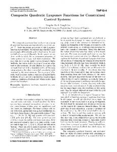
Fig. 1. Two-dimensional level set L

(1).

along the boundary of L

(1).

It is easy to see that

As to , we note that for a fixed , is a convex (this can be verified by Schur complement). function of Hence, its maximum is attained at the vertices of . It follows . The computation of these functions is easy that and straightforward, but they are not well behaved as compared . It can be verified that the level set of and with is the intersection of the ellipsoids and the level set of is the union of these ellipsoids. Both of these level sets have nonsmooth surfaces and the functions , and have nondifferentiable points.

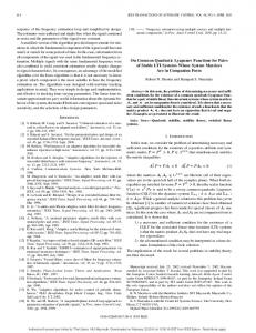
Fig. 2.

B. Computational Issues Next, we consider some computational issues with regard to . From the definition of , we have the function for some By the Schur complement, we obtain (2)

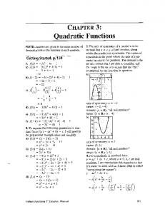
Fig. 3. Three-dimensional level set L

which is an optimization problem with linear matrix inequality (LMI) constraints and can be easily solved with the techniques in [3]. such that We see that the optimal value of is . In some situations, the optimal value of is not can be exunique. For example, this may happen if some pressed as the convex combination of other matrices in the set. Fig. 1 illustrates a two-dimensional level set which is the convex hull of three ellipsoids. Fig. 2 plots the values of as varies along the boundary in the counterclockwise direction, where the abscissa of is the angle of (from 0 to ). From Fig. 1, we see that parts

(1).

of overlap with segments of . The overlapped segments correspond to the intervals in Fig. 2, for some . Fig. 3 illustrates a three dimenwhere sional level set. It is also the convex hull of three ellipsoids. C. Special Case: Two Ellipsoids If we only have two ellipsoids, there exists a more efficient through computing the generalized eigenway to obtain values of certain matrices. In this case, we have

Denote

.


443

Proposition 1: Assume that is nonsingular. For , the function is strictly every such that convex and there exists a unique . Moreover, is a continuous function. Proof: See Appendix A.2. Remark 2: The assumption that is nonsingular is , without loss of generality. For the case where implies that either or . If , and , which is trivial. then By Proposition 1, is the unique value and hence such that . Since is continuous, is also continuous. This will be useful in Section V to our construcproperty of tion of continuous feedback laws. Here we provide a method for a given . By Propofor computing such that and . sition 1, this will give us and be given. AsProposition 2: Let is nonsingular. Let be such that sume that and . Let , and partition and as

Then,

at

if and only if

Since is generally not an invariant set, we would like to detersuch that, for any initial state in mine a maximal subset of this subset, the state trajectory of (5) will stay in it and converge to the origin. Because of the intrinsic difficulty involved in determining the maximal invariant set inside , alternative problems have been formulated such as determining the invariant ellipsoids and searching for the largest invariant ellipsoid inside . In [13], we derived a sufficient condition for checking the invariance of a given ellipsoid. This condition turns out to be also necessary for single input systems [12]. We need some notation to state the set invariance condition of [13]. Let be the set of diagonal matrices whose diagonal eleelements in . Suppose ments are either 1 or 0. There are , . Then, that each element of is labeled as . Denote . Given two matrices

is the set of matrices formed by choosing some rows from and the rest from . . The Given a positive–definite matrix , let is said to be contractively invariant if ellipsoid (6)

(3) Proof: See Appendix A.3. All the ’s satisfying (3) can be obtained by computing the where generalized eigenvalues of the matrix pair

. The invariance of can be for all is defined by replacing “ ” in (6) with “ .” Clearly, if , contractively invariant, then for every initial state is the state trajectory will converge to the origin and inside the domain of attraction. , if there Proposition 3 [11], [13]: Given an ellipsoid such that exists an

(7) By Propositions 1 and 2, has at most one generalized . If there is none in , then 0 eigenvalue in and or 1. Experience shows that computing the matrices and their generalized eigenvalues requires much less time than solving the LMI problem (2). III. INVARIANT SETS UNDER A GIVEN SATURATED LINEAR FEEDBACK Consider the open-loop system (4) is the state and is the output of satwhere urating actuators and is assumed to satisfy the bound . The state constraint is represented by a convex set , which contains the origin in its interior. It is required that the system for all . Suppose that we have a stabilizing operate in , under which the closed-loop system feedback law is (5)

, Then, is a (contractively) inand variant set. The condition in Proposition 3 is easy to check with the LMI method. To impose the state constraint, we only need to re. In the case that is a symmetric quire that for some integer polytope, there exists a matrix such that . In light of Fact 1, the requirement can be easily transformed into LMIs. In that [11]–[13], we also developed LMI methods for choosing the largest invariant ellipsoid with respect to some shape reference set, where the matrix was taken as an optimizing parameter. The shape reference set could be a polygon or a fixed ellip. In this case, the soid. It could also be a single point is the one that includes largest invariant ellipsoid inside with the maximal . By choosing different , say, , , we can obtain optimized invariant ellipsoids , . It is easy to see that the union of these ellipsoids, , is also an invariant set inside . But this union does not necessarily include the convex , . What is desired here is that the convex hull of , is also an inhull of the ellipsoids, variant set.

444


For simplicity and without loss of generality, we will con, with sider a set of invariant ellipsoids . The following theorem says that if each satisfies the condition of Proposition 3, then their convex hull, , is also invariant. , . If Theorem 2: Given a set of ellipsoids , , such that there exist matrices (8) , , then and is an invariant set. If “ ” holds for each of the aforementioned inequalities, then for every initial state , the state trajectory will converge to the origin. and . The inequalities Proof: Let in (8) are equivalent to

(9) ,

The condition

, can be written as

The inequalities in (13) and the condition (14) jointly show that is an invariant set by Proposition 3. Hence, a trajectory will stay inside of , which is a subset of starting from . Since is an arbitrary point inside , it follows that this convex hull is an invariant set. If “ ” holds for all the inequalities in (8), then we also have “ ” in (13), which guarantees that the trajectory will converge to the origin. starting form For single input systems, it was shown in [12] that the set invariance condition in Proposition 3 is also necessary. is contractively invariant, then Hence, if each ellipsoid is an invariant set inside the domain of attraction. IV. CONTROLLED INVARIANT SETS In this section, we investigate the possibility that a level set can be made invariant with controls delivered by the saturating , suppose that actuators. Given a positive–definite function is bounded and . A level the level set is said to be controlled contractively invariant if for set , there exists a , , such every that

(10) is the th row of the matrix . There exists , such that . Let and . Then, by Theorem 1, . From , we have equivalent to

where

. Consider and and

, which is

By the convexity, we have

which implies that and . , and be the th row Let of , then by (9), (10), and the convexity, we have (11) and (12) Let be rewritten as

The controlled invariance can be defined by replacing “ ” with , we have “ .” Since . Hence, if is controlled (contractively) is for all . Therefore, to deterinvariant, then , it suffices mine the controlled (contractive) invariance of . For the composite quadratic to check all the points in defined in (1), we have Lyapunov function , Theorem 3: Suppose that each of the ellipsoids , is controlled (contractively) invariant, then is controlled (contractively) invariant. Proof: We only prove controlled invariance. The controlled contractive invariance can be shown similarly. . The condition implies that for all Denote , there exists a , , such that (15) . If Now, we consider an arbitrary for some , then and follows from (15). Hence we asfor any . Then, there exist an insume that , some numbers and vectors teger , such that

. The inequalities in (11) and (12) can

(13) and

(14)

(Here, we have assumed for simplicity that is only reellipsoids. Otherwise, the ellipsoids lated to the first can be reordered to meet this assumption). Let , then by Theorem 1, . It follows that the hyperplane is at . Hence tangential to the convex set


lies between Therefore

and

445

, i.e.,

. (16)

and

We claim that contrary that

for all for some , say,

that the union is invariant. In this section, we would like to construct a continuous feedback law from these ’s such that the convex hull of the ellipsoids, , is invariant. and feedback matrices Theorem 4: Given ellipsoids , . Suppose that there exist such that and

. Suppose on the , then

(18) and be such that , where

for all . Let

which is a contradiction. Because of (16) and , the implies that touches the hyperplane equality at . Hence, the hyperplane is tangential at for every . It follows from Fact 1 that to

By assumption, there exists a

i.e., . Then,

, such that

. Let

, . Define

Then,

is (contractively) invariant under the feedback . Moreover, if the vector function is continuous, then is a continuous feedback law. Proof: In the following, we only prove the invariance of . The contractive invariance follows from similar argu. Denote and ments. Let . We see that (18) can be rewritten as

, for all . Let and by the convexity, we have

Since is an arbitrary point in , this implies that the is controlled invariant. level set If a level set is controlled contractively invariant, a simple feedback law to make it contractively invariant is (17) where is the th column of . However, due to the discontinuity of the sign function, the closed-loop system under this control may be not well behaved. For instance, the closed-loop differential equation may have no solution. It can be shown with methods in [11, Ch. 11] that there exists a positive number such that is contractively invariant under the saturated linear feedback law

This control is continuous in since both and are continuous. The value of may be however difficult to determine. In the next section, we will provide a method for constructing a controller from a set of saturated linear feedback laws. V. CONSTRUCTION OF CONTINUOUS FEEDBACK LAWS Suppose that we have a set of ellipsoids , , each of which is (contractively) invariant under a corresponding . It was shown in [11] saturated linear feedback and [15] that a switching feedback law can be constructed such

for all and vexity that (14), where the dependence on

for all alent to

and

. It follows from the con(see the proof of Theorem 2, is suppressed) and

. The previous inequality is equiv-

By Proposition 3, this inequality along with ensures that is invariant under the control , i.e., of (19) For an arbitrary , i.e.,

, let . Then, , and from Theorem 1

It follows from (19) that

This shows that

is invariant under the control of .

446


Fig. 5.

Fig. 4. Convex hull of two ellipsoids.

Let us now address the continuity of the feedback law. As we is nonsingular for all . have noted earlier, the matrix is continuous in . Since the saturation Hence, is continuous and by assumption is confunction tinuous, it follows that the feedback law is continuous. Remark 3: In Theorem 4, we assumed that the function is continuous. For the case where and is nonis continuous by Proposition 1 and can be comsingular, , as we have noted earlier, puted with Proposition 2. If could be nonunique in some special cases where one of is the convex combination of other matrices in the set. the Such special cases may be considered as degenerated. We may ’s exclude such special cases by assuming that none of the is in the convex hull of other ellipsoids. Whether this assumpis an tion will lead to the uniqueness and continuity of interesting problem and needs further study. Example: Consider system (4) with

Trajectory and the invariant set L

(1).

Fig. 6. Control signal u(t) and the Lyapunov function V (x(t)).

dotted curves. It can be verified that is nonsingular. So we can use the method in Proposition 2 to , which is guaranteed to be continuous by Propocompute sition 1. Simulation is carried out under the feedback law , where

We have designed two feedback matrices

along with two ellipsoids

and

and

, where

In Fig. 5, a trajectory starting from is plotted. Fig. 6 (in solid curve) and the composite plots the control signal (in dashed curve). quadratic function The matrices

and

maximized, where

are designed such that the value and

under guaranteed convergence rate inside and are designed such that the value The matrices maximized, where

and

is has a . is has a

under guaranteed convergence rate inside (see [11] for the detailed design method). In Fig. 4, the boundaries of the two ellipsoids are plotted in solid curves. The dotted as varies in the set . curves are the boundaries of can be seen from these The shape of

VI. CONCLUSION This paper introduced the composite quadratic Lyapunov function and showed that it is a powerful tool to handle saturation nonlinearity. The composite quadratic Lyapunov function is continuously differentiable and its level set is the convex hull of a set of ellipsoids. Using these results, we studied some set invariance properties of continuous-time linear systems with input saturation. In particular, we showed that if every ellipsoid in a set is invariant under a saturated feedback, then their convex hull is also invariant. Similar results on controlled


447

invariance have also been established. We also proposed a method to construct a continuous feedback law based on a set of saturated linear feedback laws to make the convex hull of a set of ellipsoids invariant. There still exist some interesting problems about the composite quadratic Lyapunov function. For example, the computation of this function is carried out by solving an LMI problem. motivates us to find a The simplification for the case . Also, more efficient way to compute this function for for we have only given condition for the continuity of and the condition for more general cases remains unknown. Nevertheless, the composite quadratic function is relatively easier to handle than a general nonlinear Lyapunov function and we expect to use it to study more general nonlinear systems. APPENDIX PROOFS OF THEOREM 1 AND PROPOSITIONS 1 AND 2 A. Proof of Theorem 1 , so , it suffices to show that

a) It is obvious that . Since

We first show that pose

, then there exists a , such that

Since , we have (by the Schur complement) to

This implies that each ellipsoid and planes Fact 1, we have

is between the hyperwithout touching them. By (20)

By the convexity, we should have (21) However, since the hyperplane , we also have

touches the ellipsoid

which contradicts (21). Therefore, we conclude that there exists such that . This no . proves that . Suppose that Finally, we show that . Then there exists a such that . . It follows that Combining the previous set inclusion results, we obtain

. Supand Therefore

b) Let us first establish a property about the differentiability is differenwhich will simplify the proof. Suppose that with partial derivative and let be tiable at given. Since for all , we have , we have,

. It follows that

and

that It suffices to show that for every . Let be any vector in the set . One way for the proof is to show , there exist a and a set of that for any , such that . However, this approach seems to be not easy. Instead, we will by using Fact 1. prove Suppose on the contrary that there exists an and . Then, there exists a vector such that

Let

and the hyperplane touches the ellipat only one point . It is obvious that

, which is equivalent

Recalling that by the convexity

which implies that . We next prove .

soid

be the point such that and let , then

where

can be any norm. It follows that

In view of this equality, we only need to consider those on the , . Here, we use “ ” to denote both boundary of the boundary of a set and the partial derivative. is convex, for each , there Since the set such that exists a vector (22)

448


which implies that such that

Since and

. Let

be an optimal

which implies that is differentiable at and . It follows that is the partial derivative is given by with the partial derivative given by differentiable at

, it follows that In the rest of the proof, we show that in . Since

By Fact 1, the hyperplane is tangential to the ellipsoid at . Therefore, such a vector is uniquely deter. mined by . To simplify the notation, denote Combining the aforementioned results, we have (23)

is continuous

it suffices to prove the continuity on the surface . Let with and defined as before. Then, we and . Consider have . Let

By Fact 1, we also have (24) and (25)

Then, ,

and by the foregoing proof, we have and, hence, . By Fact 1

Now, we show that

(29)

From (23), it follows that for all and , i.e.,

,

,

Since

and , we have

Since every point in can be written as and , we have

for some

such that It follows that there exists a positive number for all . Now, suppose on the is not continuous at on the surcontrary that . Then, there exists a positive number such face , there exists a that for any arbitrarily small number satisfying . Note that is fixed and can be arbitrarily small. What we will show next is that the assumption of the existence of such will cause contradiction. From above, we have

By Fact 1, we know that (26) Then, it is clear that

Recalling that

and from (24), we have (30)

Hence (27) Recalling from (22) that

,

. On the , we have

, we have (28)

Combining (26)–(28) and that

Hence, for all other hand, for all and

Hence

, we obtain Let

be chosen such that

. Then (31)


449

By assumption, there exists a such that (note that is from , which contradicts (29)). It follows from (30) that must be continuous at . (31). Therefore, Finally, we note that the partial derivative is continuous at with . B. Proof of Proposition 1 The first and the second partial derivatives of respect to are

with

Let be a matrix function. Suppose that nonsingular, then

is

(34) unit matrix and 0 to In what follows, we use to denote the denote a zero matrix of appropriate dimension. For simplicity, to denote . we use and , then we must If . From (34), we have have

which can be written as and By applying (32) and (33), we obtain a sequence of equivalent relations Since for all and is nonsingular, we have for all and . This shows that , is strictly such convex and establishes the uniqueness of . Consider . If that , then for in a neighborhood of , has a unique minimum at satisfying

Since , by implicit function theorem, is continuously differentiable at . For those such that (or 1), we have two possibilities. . Then as varies in a neighbor1) occurs in a neighborhood of hood of , . In this neighborhood of , if for , then we must have and, if some for some , then and must be . These show the continuity in a neighborhood of for this case. of . Then we have for 2) all in a neighborhood of . By the convexity, we have for all in this neighborhood of , which . also confirms the continuity of

Multiplying the matrices on both sides from left with and from right with

, we obtain

C. Proof of Proposition 2 In the proof, we will use the following algebraic fact. Supand

pose that

are square matrices. If

is (35)

nonsingular, then (32) and if

is nonsingular, then (33)

has been added to the upper-right Here, we notice that block of the right-hand side matrix. This does not change the value of the determinant. The two determinants in (35) are different only at the first column. By using the property of determinant on column addiand , we have the equation shown tion and the partition of at the top of the next page. The last equality is (3).

450


REFERENCES [1] D. S. Bernstein and A. N. Michel, “A chronological bibliography on saturating actuators,” Int. J. Robust Nonlinear Control, vol. 5, pp. 375–380, 1995. [2] F. Blanchini, “Set invariance in control—A survey,” Automatica, vol. 35, no. 11, pp. 1747–1767, 1999. [3] S. Boyd, L. El Ghaoui, E. Feron, and V. Balakrishnan, “Linear matrix inequalities in systems and control theory,” in SIAM Studies in Applied Mathematics. Philadelphia, PA: SIAM, 1994. [4] P. d’Alessandro and E. De Santis, “Controlled invariance and feedback laws,” IEEE Trans. Automat. Contr., vol. 46, pp. 1141–1146, 2001. [5] J. A. De Dona, S. O. R. Moheimani, G. C. Goodwin, and A. Feuer, “Robust hybrid control incorporating over-saturation,” Syst. Control Lett., vol. 38, pp. 179–185, 1999. [6] E. J. Davison and E. M. Kurak, “A computational method for determining quadratic Lyapunov functions for nonlinear systems,” Automatica, vol. 7, pp. 627–636, 1971. [7] E. G. Gilbert and K. T. Tan, “Linear systems with state and control constraints: The theory and application of maximal output admissible sets,” IEEE Trans. Automat. Contr., vol. 36, pp. 1008–1020, 1991. [8] P. O. Gutman and M. Cwikel, “Admissible sets and feedback control for discrete-time linear dynamical systems with bounded control and dynamics,” IEEE Trans. Auto. Contr., vol. AC-31, pp. 373–376, 1986. [9] D. Henrion, G. Garcia, and S. Tarbouriech, “Piecewise-linear robust control of systems with input constraints,” Euro. J. Control, vol. 5, pp. 157–166, 1999. [10] H. Hindi and S. Boyd, “Analysis of linear systems with saturating using convex optimization,” in Proc. 37th IEEE Conf. Decision Control, Tampa, FL, 1998, pp. 903–908. [11] T. Hu and Z. Lin, Control Systems With Actuator Saturation: Analysis and Design. Boston, MA: Birkhäuser, 2001. , “Exact characterization of invariant ellipsoids for linear systems [12] with saturating actuators,” IEEE Trans. Automat. Contr., vol. 47, pp. 164–169, 2002. [13] T. Hu, Z. Lin, and B. M. Chen, “An analysis and design method for linear systems subject to actuator saturation and disturbance,” Automatica, vol. 38, pp. 351–359, 2002. [14] T. Hu, Z. Lin, and L. Qiu, “Stabilization of exponentially unstable linear systems with saturating actuators,” IEEE Trans. Automat. Contr., vol. 46, pp. 973–979, 2001. [15] T. Hu, Z. Lin, and Y. Shamash, “Semi-global stabilization with guaranteed regional performance of linear systems subject to actuator saturation,” Syst. Control Lett., vol. 43, no. 3, pp. 203–210, 2001. [16] M. Johansson and A. Rantzer, “Computation of piecewise quadratic Lyapunov functions for hybrid systems,” IEEE Trans. Automat. Contr., vol. 43, pp. 555–559, Apr. 1998. [17] Z. Lin, Low Gain Feedback. London, U.K.: Springer-Verlag, 1998. [18] Z. Lin and A. Saberi, “Semi-global exponential stabilization of linear systems subject to ’input saturation’ via linear feedbacks,” Syst. Control Lett., vol. 21, pp. 225–239, 1993. [19] K. A. Loparo and G. L. Blankenship, “Estimating the domain of attraction of of nonlinear feedback systems,” IEEE Trans. Automat. Contr., vol. AC-23, pp. 602–607, Apr. 1978. [20] D. Liu and A. N. Michel, Dynamical Systems with Saturation Nonlinearities. London, U.K.: Springer-Verlag, 1994. [21] D. Q. Mayne, J. B. Rawlings, C. V. Rao, and P. O. M. Scokaert, “Constrained model predictive control: Stability and optimality,” in Automatica, vol. 36, 2000, pp. 789–814. [22] D. Q. Mayne, “Control of constrained dynamic systems,” Euro. J. Control, vol. 7, pp. 87–99, 2001. [23] B. E. A. Milani, “Piecewise-affine Lyapunov functions for discrete-time linear systems with saturating controls,” in Proc. Amer. Control Conf., Arlington, VA, 2001, pp. 4206–4211.

[24] H. J. Sussmann, E. D. Sontag, and Y. Yang, “A general result on the stabilization of linear systems using bounded controls,” IEEE Trans. Automat. Contr., vol. 39, pp. 2411–2425, 1994. [25] R. Suarez, J. Alvarez-Ramirez, and J. Solis-Daun, “Linear systems with bounded inputs: Global stabilization with eigenvalue placement,” Int. J. Robust Nonlinear Control, vol. 7, pp. 835–845, 1997. [26] A. R. Teel, “Global stabilization and restricted tracking for multiple integrators with bounded controls,” Syst. Control Lett., vol. 18, pp. 165–171, 1992. , “Linear systems with input nonlinearities: Global stabilization by [27] -type controllers,” Int. J. Robust Nonlinear scheduling a family of Control, vol. 5, pp. 399–441, 1995. [28] G. F. Wredenhagen and P. R. Belanger, “Piecewise-linear lq control for systems with input constraints,” Automatica, vol. 30, pp. 403–416, 1994.

H

Tingshu Hu (S’99–SM’01) was born in Sichuan, China, in 1966. She received the B.S. and M.S. degrees in electrical engineering from Shanghai Jiao Tong University, Shanghai, China, and the Ph.D. degree in electrical engineering from University of Virginia, Charlottesville, in 1985, 1988, and 2001, respectively. Her research interests include nonlinear systems, robust control and magnetic bearing systems. In these areas, she has published several papers. She is also a coauthor (with Z. Lin) of the book Control Systems with Actuator Saturation: Analysis and Design (Boston, MA: Birkhäuser, 2001). Dr. Hu is currently an Associate Editor on the Conference Editorial Board of the IEEE Control Systems Society.

Zongli Lin (S’89–M’90–SM’98) received the B.S. degree in mathematics and computer science from Xiamen University, Xiamen, China, the M.E. degree in automatic control from the Chinese Academy of Space Technology, Beijing, China, and the Ph.D. degree in electrical and computer engineering from Washington State University, Pullman, in 1983, 1989, and 1994, respectively. He is currently an Associate Professor with the Department of Electrical and Computer Engineering, the University of Virginia, Charlottesville. Previously, he has worked as a Control Engineer at the Chinese Academy of Space Technology and as an Assistant Professor with the Department of Applied Mathematics and Statistics, the State University of New York at Stony Brook. His current research interests include nonlinear control, robust control, and modeling and control of magnetic bearing systems. In these areas, he has published several papers. He is also the author of the book Low Gain Feedback (London, U.K.: Springer-Verlag, 1998) and a coauthor (with T. Hu) of the recent book Control Systems with Actuator Saturation: Analysis and Design (Boston, MA: Birkhäuser, 2001). Dr. Lin currently serves as an Associate Editor of the IEEE TRANSACTIONS ON AUTOMATIC CONTROL. He is also a Member of the IEEE Control Systems Society’s Technical Committee on Nonlinear Systems and Control, and heads its Working Group on Control with Constraints. He was the recipient of a U.S. Office of Naval Research Young Investigator Award.