Compositionality in Synchronous Data Flow: Modular Code ... - DTIC

Compositionality in Synchronous Data Flow: Modular Code Generation from Hierarchical SDF Graphs

Stavros Tripakis Dai Bui Bert Rodiers Edward A. Lee

Electrical Engineering and Computer Sciences University of California at Berkeley Technical Report No. UCB/EECS-2009-143 http://www.eecs.berkeley.edu/Pubs/TechRpts/2009/EECS-2009-143.html

October 20, 2009

Form Approved OMB No. 0704-0188

Report Documentation Page

Public reporting burden for the collection of information is estimated to average 1 hour per response, including the time for reviewing instructions, searching existing data sources, gathering and maintaining the data needed, and completing and reviewing the collection of information. Send comments regarding this burden estimate or any other aspect of this collection of information, including suggestions for reducing this burden, to Washington Headquarters Services, Directorate for Information Operations and Reports, 1215 Jefferson Davis Highway, Suite 1204, Arlington VA 22202-4302. Respondents should be aware that notwithstanding any other provision of law, no person shall be subject to a penalty for failing to comply with a collection of information if it does not display a currently valid OMB control number.

1. REPORT DATE

3. DATES COVERED 2. REPORT TYPE

20 OCT 2009

00-00-2009 to 00-00-2009

4. TITLE AND SUBTITLE

5a. CONTRACT NUMBER

Compositionality in Synchronous Data Flow: Modular Code Generation from Hierarchical SDF Graphs

5b. GRANT NUMBER 5c. PROGRAM ELEMENT NUMBER

6. AUTHOR(S)

5d. PROJECT NUMBER 5e. TASK NUMBER 5f. WORK UNIT NUMBER

7. PERFORMING ORGANIZATION NAME(S) AND ADDRESS(ES)

University of California at Berkeley,Department of Electrical Engineering and Computer Sciences,Berkeley,CA,94720 9. SPONSORING/MONITORING AGENCY NAME(S) AND ADDRESS(ES)

8. PERFORMING ORGANIZATION REPORT NUMBER

10. SPONSOR/MONITOR’S ACRONYM(S) 11. SPONSOR/MONITOR’S REPORT NUMBER(S)

12. DISTRIBUTION/AVAILABILITY STATEMENT

Approved for public release; distribution unlimited 13. SUPPLEMENTARY NOTES 14. ABSTRACT

Hierarchical SDF models are not compositional: a composite SDF actor cannot be represented as an atomic SDF actor without loss of information that can lead to deadlocks. Motivated by the need for incremental and modular code generation from hierarchical SDF models, we introduce in this paper DSSF profiles. This model forms a compositional abstraction of composite actors that can be used for modular compilation. We provide algorithms for automatic synthesis of non-monolithic DSSF profiles of composite actors given DSSF profiles of their sub-actors. We show how different tradeoffs can be explored when synthesizing such profiles, in terms of modularity (keeping the size of the generated DSSF profile small) versus reusability (preserving information necessary to avoid deadlocks) as well as algorithmic complexity. We show that our method guarantees maximal reusability and report on a prototype implementation. 15. SUBJECT TERMS 16. SECURITY CLASSIFICATION OF: a. REPORT

b. ABSTRACT

c. THIS PAGE

unclassified

unclassified

unclassified

17. LIMITATION OF ABSTRACT

18. NUMBER OF PAGES

Same as Report (SAR)

22

19a. NAME OF RESPONSIBLE PERSON

Standard Form 298 (Rev. 8-98) Prescribed by ANSI Std Z39-18

Copyright © 2009, by the author(s). All rights reserved. Permission to make digital or hard copies of all or part of this work for personal or classroom use is granted without fee provided that copies are not made or distributed for profit or commercial advantage and that copies bear this notice and the full citation on the first page. To copy otherwise, to republish, to post on servers or to redistribute to lists, requires prior specific permission.

Compositionality in Synchronous Data Flow: Modular Code Generation from Hierarchical SDF Graphs∗ Stavros Tripakis, Dai Bui, Bert Rodiers and Edward A. Lee Department of Electrical Engineering and Computer Sciences University of California, Berkeley stavros, daib, [email protected] October 20, 2009

Abstract Hierarchical SDF models are not compositional: a composite SDF actor cannot be represented as an atomic SDF actor without loss of information that can lead to deadlocks. Motivated by the need for incremental and modular code generation from hierarchical SDF models, we introduce in this paper DSSF profiles. This model forms a compositional abstraction of composite actors that can be used for modular compilation. We provide algorithms for automatic synthesis of non-monolithic DSSF profiles of composite actors given DSSF profiles of their sub-actors. We show how different tradeoffs can be explored when synthesizing such profiles, in terms of modularity (keeping the size of the generated DSSF profile small) versus reusability (preserving information necessary to avoid deadlocks) as well as algorithmic complexity. We show that our method guarantees maximal reusability and report on a prototype implementation.

1

Introduction

Programming languages have been constantly evolving over the years, from assembly, to structural programming, to object-oriented programming, etc. Common to this evolution is the fact that new programming models provide mechanisms and notions that are more abstract, that is, remote from the actual implementation, but better suited to the programmer’s intuition. Raising the level of abstraction results in undeniable benefits in productivity. But it is more than just building systems faster or cheaper. It also allows to create systems that could not have been conceived otherwise, simply because of too high complexity. Modeling languages with built-in concepts of concurrency, time, I/O interaction, and so on, are particularly suitable in the domain of embedded systems. Indeed, languages such as Simulink, UML or SystemC, and corresponding tools, are particularly popular in this domain, for various applications. The tools provide mostly modeling and simulation, but often also code generation and static analysis or verification capabilities, which are increasingly important in an industrial setting. We believe that this tendency will continue, to the point where modeling languages of today will become the programming languages of tomorrow, at least in the embedded software domain. Synchronous (or Static) Data Flow (SDF) models [6] is a successful model in this domain, particularly for signal processing and multimedia applications. This model has been extensively studied over the years, in particularly regarding efficient scheduling and implementation (e.g., see [1, 10]). In this paper we consider hierarchical SDF models, where an SDF graph can be encapsulated into a composite SDF actor. This actor ∗ This work is supported by the Center for Hybrid and Embedded Software Systems (CHESS) at UC Berkeley, which receives support from the National Science Foundation (NSF awards #0720882 (CSR-EHS: PRET) and #0720841 (CSR-CPS)), the U.S. Army Research Office (ARO #W911NF-07-2-0019), the U.S. Air Force Office of Scientific Research (MURI #FA9550-06-0312), the Air Force Research Lab (AFRL), the State of California Micro Program, and the following companies: Agilent, Bosch, Lockheed-Martin, National Instruments, Thales and Toyota.

1

can then be connected with other SDF actors, further encapsulated, and so on, to form a hierarchy of SDF actors of arbitrary depth. This is essential for compositional modeling, which allows to design systems in a modular, scalable way, enhancing readability and allowing to master complexity in order to build larger designs. Hierarchical SDF models are part of a number of modeling environments, including the Ptolemy II framework [3]. The problem we solve in this paper is modular code generation for hierarchical SDF models. Modular means that code is generated for a given composite SDF actor P independently from context, that is, independently from which graphs P is going to be used in. Moreover, once code is generated for P , then P can be seen as an atomic (non-composite) actor, that is, a “black box” without access to its internal structure. Modular code generation can be paralleled to separate compilation, which is available in most standard programming languages: the fact that one does not need to compile an entire program in one shot, but can compile files, classes, or other units, separately, and then combine them (e.g., by linking) to a single executable. This is obviously a key capability for a number of reasons, ranging from incremental compilation (compiling only the parts of a large program that have changed), to dealing with IP (intellectual property) concerns (having access to object code only and not to source code). We want to do the same for SDF models. Moreover, in the context of a system like Ptolemy II, in addition to the benefits mentioned above, modular code generation is also useful for speeding-up simulation: replacing entire sub-trees of a large hierarchical model by a single actor for which code has been automatically generated and pre-compiled, removes the overhead of executing all actors in the sub-tree individually. Our work extends the ideas of modular code generation for synchronous block diagrams (SBDs), introduced in [8, 7]. In particular, we borrow their notion of profile which characterizes a given actor. Modular code generation then essentially becomes a profile synthesis problem: how to synthesize a profile for composite actors, based on the profiles of its internal actors. In SBDs, profiles are essentially DAGs (directed acyclic graphs) that capture the dependencies between inputs and outputs of a block, at the same synchronous round. In general, not all outputs depend on all inputs, which allows feedback loops with unambiguous semantics to be built. For instance, in a unit delay block the output does not depend on the input at the same clock cycle, therefore this block “breaks” dependency cycles when used in feedback loops. The question is, what is the right model for profiles of SDF graphs. We answer this question in this paper. For SDF graphs, profiles turn out to be more interesting than simple DAGs. SDF profiles are essentially SDF graphs themselves, but with the ability to associate multiple producers and/or consumers with a single FIFO queue. Sharing FIFOs among different actors generally results in non-deterministic models, however, in our case, we can guarantee that actors that share queues are always fired in a deterministic order. We call this model deterministic SDF with shared FIFOs (DSSF). DSSF allows, in particular, to decompose the firing of a composite actor into an arbitrary number of firing functions that may consume tokens from the same input port or produce tokens to the same output port (an example is shown in Figure 4). Having multiple firing functions allows to decouple firings of different internal actors of the composite actor, so that deadlocks are avoided when the composite actor is embedded in a given context. Our method guarantees maximal reusability [8], i.e., the absence of deadlock in any context where the corresponding “flat” (non-hierarchical) SDF graph is deadlock-free. We show how to perform profile synthesis for SDF graphs automatically. This means synthesize for a given composite actor a profile, in the form of a DSSF graph, given the profiles of its internal actors (also DSSF graphs). This process involve multiple steps, among which are the standard rate analysis and deadlock detection procedures used to check whether a given SDF graph can be executed infinitely often without deadlock and with bounded queues [6]. In addition to these steps, SDF profile synthesis involves unfolding a DSSF graph (i.e., replicating actors in the graph according to their relative rates produced by rate analysis) to produce a DAG that captures the dependencies between the different consumptions and productions of tokens at the same port. This is interesting because it allows to re-use for our purposes the DAG clustering methods proposed for SBDs [8, 7]. We use DAG clustering in order to group together firing functions of internal actors and synthesize a small (hopefully minimal) number of firing functions for the composite actor. These determine precisely the profile of the latter. Keeping the number of firing functions small is essential,

2

because it results in further compositions of the actor being more efficient, thus allowing the process to scale to arbitrary levels of hierarchy. The rest of this paper is organized as follows. Section 2 discusses related work. Section 3 reviews (hierarchical) SDF graphs. Section 4 reviews rate analysis and deadlock detection for flat SDF graphs. Section 5 reviews modular code generation for SBDs which we build upon. Section 6 introduces DSSF as profiles for SDF graphs. Section 7 elaborates on the profile synthesis procedure, detailing each step except DAG clustering, which is detailed in Section 8. Section 9 presents a prototype implementation. Section 10 presents the conclusions and discusses future work.

2

Related Work

Despite extensive work on code generation from SDF models (e.g., see [1], there is little existing work that addresses compositionality and modular code generation. [5] proposes abstraction methods that reduce the size of SDF graphs, thus facilitating throughput and latency analysis. His goal is to have a conservative abstraction in terms of these performance metrics, whereas our goal here is to preserve input-output dependencies to avoid deadlocks during further composition. Non-compositionality of SDF due to potential deadlocks has been observed in earlier works such as [9], where the objective is schedule SDF graphs on multiple processors. This is done by partitioning the SDF graph into multiple sub-graphs, each of which is scheduled on a single processor. This partitioning (also called clustering, but different from DAG clustering that we use in this paper, see below) may result in deadlocks, and the so-called “SDF composition theorem” given in [9] provides a sufficient condition so that no deadlock is introduced. More recently, [4] also identify the problem of non-compositionality and propose Cluster Finite State Machines (CFSMs) as a representation of composite SDF. They show how to compute a CFSM for a composite SDF actor that contains standard, atomic, SDF sub-actors, however, they do not show how a CFSM can be computed when the sub-actors are themselves represented as CFSMs. This indicates that this approach may not generalize to more than one level of hierarchy. Our approach works for arbitrary depths of hierarchy. Another difference between the above work and ours is on the representation models, namely, CFSM vs. DSSF. CFSM is a state-machine model, where transitions are annotated with guards checking whether a sufficient number of tokens is available in certain input queues. DSSF, on the other hand, is a data flow model, only slightly more general than SDF. This allows to re-use many of the techniques developed for standard SDF graphs, for instance, rate analysis and deadlock detection, with minimal adaptation. Finally, we should emphasize our DAG clustering algorithms solve a different problem than the clustering methods used in [9, 4] and other works in the SDF scheduling literature. Our clustering algorithms operate on plain DAGs, as do the clustering algorithms originally developed for SBDs [8, 7]. On the other hand, clustering in [4, 9] is done directly at the SDF level, by grouping SDF actors and replacing them by a single SDF actor (e.g., see Figure 4 in [4]). This, in our terms, corresponds to monolithic clustering, which is not compositional.

3

Hierarchical SDF Graphs

A synchronous (or static) dataflow (SDF) graph [6] consists of a set of nodes, called actors1 connected through a set of directed edges. Each actor has a set of input ports (possibly zero) and a set of output ports (possibly zero). An edge connects an output port y of an actor A to an input port x of an actor B (B 1 It is useful to distinguish between actor types and actor instances. Indeed, an actor can be used in a given graph multiple times. For example, an actor of type Adder, that computes the arithmetic sum of its inputs, can be used multiple times in a given graph. In this case, we say that the Adder is instantiated multiple times. Each “copy” is an actor instance. In the rest of the paper, we often omit to distinguish between type and instance when we refer to an actor, when the meaning is clear from context.

3

can be the same as A). An output port can be connected to a single input port, and vice versa.2 Such an edge represents a FIFO (first-in, first-out) queue, that stores tokens that the source actor A produces when it fires. The tokens are removed and consumed by the destination actor B when it fires. Queues are of unbounded size in principle. In practice, however, we are interested in SDF graphs that can execute forever using bounded queues. Actors are either atomic or composite. A composite actor encapsulates an SDF graph as shown in Figure 1. P is a composite actor while A and B are atomic actors. Composite actors can themselves be encapsulated in new composite actors, thus forming a hierarchical model of arbitrary depth. Each port of an atomic actor has an associated token rate, a positive integer number, which specifies how many tokens (i.e., data values) are consumed from or produced to each port every time the actor fires. In the example of Figure 1, A consumes one token from its single input port and produces two tokens to its single output port. B consumes three tokens and produces one token. Each port of an atomic also has a given data type (integer, boolean, ...) and connections can only be done among ports with compatible data types, as in a standard typed programming language. Composite actors do not have token rate or data type annotations on their ports. They inherit this information from their internal actors, as we will explain in this paper.

P 1

2

3

1

A

B

Figure 1: Example of a hierarchical SDF graph.

SDF graphs can be open or closed. A graph is closed if all its ports are connected; otherwise it is open. The graph shown in Figure 1 is open because the ports of P are not connected. The graph shown in Figure 2 is closed. This latter graph also illustrates another element of SDF notation, namely, initial tokens: the edge from the output port of Q to the input port of P is annotated with two black dots which means there are initially two tokens in the queue from Q to P . Likewise, there is one initial token in the queue from P to Q.

P 3

2 Q

Figure 2: Using the composite actor P of Figure 1 in an SDF graph with feedback and initial tokens.

An SDF graph is flat if it contains only atomic actors. A flattening process can be applied to turn a hierarchical SDF graph into a flat graph, by removing composite actors and replacing them with their internal graph, while making sure to re-institute any connections that would be otherwise lost. For example, flattening the hierarchical SDF graph of Figure 2 produces the (flat) SDF graph of Figure 3. 2 Implicit fan-in or fan-out is not allowed, however, it can be implemented explicitly, using actors. For example, an actor that consumes an input token and replicates to each of its output ports models fan-out.

4

1

2

3

1

A

B

3

2 Q

Figure 3: After flattening the SDF graph of Figure 2.

4

Analysis of SDF Graphs

The SDF analysis methods proposed in [6] allow to check whether a given SDF graph has a periodic admissible schedule (PAS). Existence of a PAS guarantees two things: first, that the actors in the graph can fire infinitely often without deadlock; and second, that only bounded queues are required to store intermediate tokens produced during the firing of these actors. We review these analysis methods here, because we are going to use them for modular code generation (Section 7).

4.1

Rate Analysis

Rate analysis seeks to determine if the token rates in a given SDF graph are consistent: if this is not the case, then the graph cannot be executed infinitely often with bounded queues. We illustrate the analysis in the simple example of Figure 1. The reader is referred to [6] for the details. We wish to analyze the internal graph of P , consisting of actors A and B. This is an open graph, and we will ignore the unconnected ports for the rate analysis. Suppose A is fired rA times for every rB times that B is fired. Then, in order for the queue between A and B to remain bounded, it has to be the case that: rA · 2 = rB · 3 that is, the total number of tokens produced by A equals the total number of tokens consumed by B. The above balance equation has a non-trivial (i.e., non-zero) solution: rA = 3 and rB = 2. This means that this SDF graph is indeed consistent. In general, for larger and more complex graphs, the same analysis can be performed, which results in solving a system of multiple balance equations. If the system has a non-trivial solution then the graph is consistent, otherwise it is not. At the end of rate analysis, a repetition vector (r1 , ..., rn ) is produced that specifies the number ri of times that every actor Ai in the graph fires with respect to other actors. This vector is used in the subsequent step of deadlock analysis.

4.2

Deadlock Analysis

Having a consistent graph is a necessary, but not sufficient condition for infinite execution: the graph might still contain deadlocks that arise because of absence of enough initial tokens. Deadlock analysis ensures that this is not the case. The method works as follows. For every directed edge ei in the SDF graph, an integer counter bi is maintained, representing the number of tokens in the FIFO queue associated with ei . Counter bi is initialized to the number of initial tokens present in ei (zero if no such tokens are present). For every actor A in the SDF graph, an integer counter cA is maintained, representing the number of remaining times that A should fire. Counter cA is initialized to rA , where rA is the repetition value for A in the repetition vector. A tuple consisting of all above counters is called a configuration v. A transition from a configuration v to a new configuration v 0 happens by firing an actor A, provided A is enabled at v, i.e., all its input queues have enough tokens. Then, the queue counters are updated, and counter cA is decremented by 1. If a configuration is reached where all actor counters are 0, there is no deadlock, otherwise, there is one. Notice that a single path needs to be explored, so this is not a costly method (i.e., not a full-blown reachability 5

analysis). In fact, at most Σni=1 ri steps are required to complete deadlock analysis, where (r1 , ..., rn ) is the solution to the balance equations. We illustrate deadlock analysis with an example. Consider the SDF graph of Figure 2 and suppose P is an atomic actor, with input/output token rates 3 and 2, respectively. Rate analysis then gives rP = rQ = 1. Let the edges from P to Q and from Q to P be denoted e1 and e2 , respectively. Deadlock analysis then starts with configuration v0 = (cP = 1, cQ = 1, b1 = 1, b2 = 2). P is not enabled at v0 because it needs 3 input tokens but be2 = 2. Q is not enabled at v0 either because it needs 2 input tokens but be1 = 1. Thus v0 is a deadlock. Now, suppose instead of 2 initial tokens, edge e2 had 3 initial tokens. Then, we would have as initial configuration v1 = (cP = 1, cQ = 1, b1 = 1, b2 = 3). In this case, deadlock analysis can proceed: P

Q

v1 → (cP = 0, cQ = 1, b1 = 3, b2 = 0) → (cP = 0, cQ = 0, b1 = 1, b2 = 3). Since a configuration is reached where cP = cQ = 0, there is no deadlock.

4.3

Transformation of SDF to Homogeneous SDF

A homogeneous SDF graph is an SDF graph where all token rates are equal (and without loss in generality, can be assumed to be equal to 1). Any consistent SDF graph can be transformed to an equivalent homogeneous SDF graph using an unfolding process [6, 9, 10]. This process consists in replicating each actor in the SDF as many times as specified in the repetition vector. This subsequently allows to identify explicitly the input/output dependencies of different productions and consumptions at the same output or input port. Examples of this process are presented in Section 7.4, where we generalize the process to DSSF graphs.

5

Modular Code Generation Framework

As mentioned in the introduction, our modular code generation framework for SDF builds upon the work of [8, 7]. A fundamental element of the framework is the notion of profiles. Every SDF actor has an associated profile. The profile can be seen as an interface, or summary, that captures the essential information about the actor. Atomic actors have predefined profiles. Profiles of composite actors are synthesized automatically, as shown in Section 7. A profile contains, among other things, a set of firing functions, that, together, implement firing of an actor. In the simple case, an actor may have a single firing function. For example, actors A, B of Figure 1 may each have a single firing function A.fire(input x[1]) output (y[2]); B.fire(input x[3]) output (y[1]); The above signatures specify that A.fire takes as input 1 token at input port x and produces as output 2 tokens at output port y, and similarly for B.fire. In general, however, an actor may have more than one firing function in its profile. This is necessary in order to avoid monolithic code, and instead produce code that achieves maximal reusability, as is explained in Section 7.3. The implementation of a profile contains, among other things, the implementation of each of the firing functions listed in the profile as a sequential program in a language such as C++ or Java. We will show how to automatically generate such implementations of SDF profiles in Section 7.7. Modular code generation is then the following process: • given a composite actor P , its internal graph, and profiles for every internal actor of P , • synthesize automatically a profile for P and an implementation of this profile. Note that a given actor may have multiple profiles, each achieving different tradeoffs, for instance, in terms of modularity (size of the profile) and reusability (ability to use the profile in as many contexts as possible). We illustrate such tradeoffs in the sequel.

6

6

SDF Profiles

The profile of an SDF actor is called an SDF profile. An SDF profile is essentially a flat SDF graph, with the difference that whereas shared FIFOs are explicitly prohibited in SDF graphs, they are allowed in SDF profiles. Sharing FIFOs among different actors generally results in non-deterministic models, however, in our case, we can guarantee that actors that share queues are always fired in a deterministic order. We call deterministic SDF graphs with shared FIFOs DSSF graphs. An example is shown in Figure 4. This figure shows two possible profiles for the composite actor P of Figure 1. We will see how these profiles can be synthesized automatically in Section 7. We will also see that these two profiles have different properties. In particular, they represent different pareto points in the modularity vs. reusability tradeoff (Section 7.3).

2

1 P.f1

3

2

1

1

1

1

P.f 1

1 P.f2

Figure 4: Two profiles for the composite actor P of Figure 1. The actors of an SDF profile represent firing functions. They are drawn as circles instead of squares to distinguish SDF profiles from SDF graphs. The left-most profile shown in Figure 4 contains a single actor, denoted P.f , which corresponds to a single firing function P.fire. Profiles that contain a single firing function are called monolithic. The right-most profile shown in Figure 4 contains two actors, P.f1 and P.f2 , corresponding to two firing functions, P.fire1 and P.fire2: this is a non-monolithic profile. This profile also has two shared FIFOs, one connecting the input port to the two actors, and another from the two actors to the output port. Shared FIFOs are depicted as squares in the figure. Non-shared FIFOs, i.e., standard SDF edges, are a special case of shared FIFOs in the sense that they have a unique writer and a unique reader. Such edges are drawn without the square. An example is the edge from P.f1 to P.f2 . This edge encodes a dependency, namely, the fact that P.fire1 must be called before P.fire2. The edge from P.f2 to P.f1 encodes the fact that P.fire1 can be called for a second time only after the first call to P.fire2. Together these edges impose a total order on the firing of these two functions, which results in deterministic handling of tokens in the shared input and output FIFOs. Unless explicitly mentioned otherwise, in the examples that follow we assume that atomic blocks have monolithic profiles.

7

Modular Code Generation Steps

As mentioned above, modular code generation takes as input a composite actor P , its internal graph, and profiles for every internal actor of P , and produces as output a profile for P and an implementation of this profile. This is done in a number of steps, detailed below.

7.1

Connecting the SDF Profiles

The first step consists in connecting the SDF profiles of internal actors of P . This is done simply as dictated by the connections found in the internal graph of P . The result is a flat DSSF graph, called the internal DSSF graph of P . We illustrate this through an example. Consider the composite actor P shown in Figure 1. Suppose both its internal actors A and B have monolithic profiles, with A.f and B.f representing A.fire

7

and B.fire, respectively. Then, by connecting these monolithic profiles we obtain the internal DSSF graph shown in Figure 5.

x

1

2

3

A.f

1 B.f

y

Figure 5: Internal DSSF graph of composite actor P of Figure 1. A more elaborate example of connection is shown in Figure 6. Here, we are connecting the profiles of internal actors P and Q of the (closed) graph shown in Figure 2. Actor Q is assumed to have a monolithic profile. Actor P has two possible profiles, shown in Figure 4. Both possible connections are shown in Figure 6.

2

1 P.f1

3

2

1

1

1

1

P.f 1 3

1 P.f2

2 Q.f 3

2 Q.f

Figure 6: Connecting the two profiles of actor P shown in Figure 4 and a monolithic profile of actor Q, according to the graph of Figure 2.

7.2

Rate Analysis with SDF Profiles

This step is similar to the rate analysis process described in Section 4.1, except that it is performed on the internal DSSF graph produced by the connection step, instead of an SDF graph. This presents no major challenges, however, and the method is essentially the same as the one proposed in [6]. Let us illustrate the process here, for the DSSF graph shown to the right of Figure 6. We associate repetition variables rp1 , rp2 , and rq , respectively, to P.f1 , P.f2 and Q. Then, we have the following balance equations: rp1 · 1 + rp2 · 1

= rq · 2

rq · 3

= rp1 · 2 + rp2 · 1

rp1 · 1

= rp2 · 1

As this has a non-trivial solution (e.g., rp1 = rp2 = rq = 1), this graph is consistent, i.e., rate analysis succeeds in this example. If the rate analysis step fails the graph is rejected. Otherwise, we proceed with the deadlock analysis step.

7.3

Deadlock Analysis with SDF Profiles

Success of the rate analysis step is a necessary, but not sufficient, condition in order for a graph to have a PAS. Deadlock analysis is used to ensure that this is the case. Deadlock analysis is performed on the internal 8

DSSF graph produced by the connection step. It is done in the same way as the deadlock detection process described in Section 4.2. We illustrate this on the two examples of Figure 6. Consider first the DSSF graph to the left of Figure 6. There are two queues in this graph: a queue from P.f to Q.f , and a queue from Q.f to P.f . Denote the former by b1 and the latter by b2 . Initially, b1 has 1 token, whereas b2 has 2 tokens. P.f needs 3 tokens to fire but only 2 are available in b2 , thus P.f cannot fire. Q.f needs 2 tokens but only 1 is available in b1 , thus Q.f cannot fire either. Therefore there is a deadlock already at the initial state, and this graph is rejected. Now consider the DSSF graph to the right of Figure 6. There are four queues in this graph: a queue from P.f1 and P.f2 to Q.f , a queue from Q.f to P.f1 and P.f2 , a queue from P.f1 to P.f2 , and a queue from P.f2 to P.f1 . Denote these queues by b1 , b2 , b3 , b4 , respectively. Initially, b1 has 1 token, b2 has 2 tokens, b3 is empty and b4 has 1 token. P.f1 needs 2 tokens to fire and 2 tokens are indeed available in b2 , thus P.f can fire and the initial state is not a deadlock. Deadlock analysis gives: (cp1 = 1, cp2 = 1, cq = 1, b1 = 1, b2 = 2, b3 = 0, b4 = 1) (cp1 = 0, cp2 = 1, cq = 1, b1 = 2, b2 = 0, b3 = 1, b4 = 0) (cp1 = 0, cp2 = 1, cq = 0, b1 = 0, b2 = 3, b3 = 1, b4 = 0) (cp1 = 0, cp2 = 0, cq = 0, b1 = 1, b2 = 2, b3 = 0, b4 = 1)

P.f1

→

Q.f

→

P.f2

→

Therefore, deadlock analysis succeeds (no deadlock is detected). This example illustrates the tradeoff between modularity and reusability. For the same composite actor P , two profiles can be generated, as shown in Figure 4. These profiles achieve different tradeoffs. The monolithic profile shown to the left of the figure is more modular (i.e., smaller) than the non-monolithic one shown to the right. The latter is more reusable than the monolithic one, however: indeed, it can be reused in the graph with feedback shown in Figure 2, where the monolithic one cannot be used, because it creates a deadlock. Note that if we flatten the graph of Figure 2, that is, remove composite actor P and replace it with its internal graph of atomic actors A and B, then the resulting graph has a PAS, i.e., exhibits no deadlock. This shows that deadlock is a result of using the monolithic profile, and not a problem with the graph itself. Of course, flattening is not an attractive proposition, because of scalability as well as IP issues, as we explained in the introduction. If the deadlock analysis step fails then the graph is rejected. Otherwise, we proceed with the unfolding step.

7.4

Unfolding with SDF Profiles

This step takes as input the internal DSSF graph produced by the connection step, as well as the repetition vector produced by the rate analysis step. It produces as output a DAG (directed acyclic graph) that captures the input-output dependencies of the DSSF. The DAG is computed in two steps. First, the DSSF graph is unfolded, by replicating each node in it as many times as specified in the repetition vector. These replicas represent the different firings of the corresponding actor. For this reason, the replicas are ordered: dependencies are added between them to represent the fact that the first firing comes before the second firing, the second before the third, and so on. The input and output ports of the actors are also replicated. Finally, for every edge of the original DSSF, a shared FIFO is created in the unfolded graph. The process is illustrated in Figure 7, for the internal DSSF graph of Figure 5. Rate analysis in this case produces the repetition vector (rA = 3, rB = 2). Therefore A.f is replicated 3 times and B.f is replicated 2 times. In this example there is a single edge between A.f and B.f , therefore, the unfolded graph contains a single shared FIFO. In the second and final step of unfolding, the DAG is produced, by computing dependencies between the replicas. This is done by separately computing dependencies between replicas that are connected to a given FIFO, and repeating the process for every FIFO. We first explain the process for non-shared FIFOs, i.e., standard SDF edges, such as the one between A and B in the DSSF of Figure 5. Let A→B be such an edge. 9

x1 x2

1

1

A.f 1 2 A.f 2

3 B.f 1 1

y1

1

y2

2 2 3 B.f

x3

1

A.f 3

2

Figure 7: First step of unfolding the DSSF graph of Figure 5: replicating nodes and creating a shared FIFO.

Suppose the edge has n initial tokens, A produces k tokens each time it fires, and B consumes m tokens each time it fires. Then the j-th occurrence of B depends on the i-th occurrence of A iff: n + (i − 1) · k < j · m

(1)

For the example of Figure 5, this gives the DAG shown in Figure 8.

x1

A.f 1

x2

B.f 1

y1

B.f 2

y2

A.f 2

x3

A.f 3

Figure 8: Unfolding the DSSF graph of Figure 5 produces the IODAG shown here.

In the general case, a FIFO queue in the internal DSSF of P may be shared by multiple producers and multiple consumers. Consider such a shared FIFO between a set of producers A1 , ..., Aa and a set of consumers B1 , ..., Bb . Let kh be the number of tokens produced by Ah , for h = 1, ..., a. Let mh be the number of tokens consumed by Bh , for h = 1, ..., b. Let n be the number of initial tokens in the queue. By construction (see Section 7.6) there is a total order A1 →A2 → · · · →Aa on the producers and a total order 1 1 B1 →B2 → · · · →Bb on the consumers. As this is encoded with standard SDF edges of the form Ai → Ai+1 , this also implies that during rate analysis the rates of all producers will be found equal, and so will the rates of all consumers. Then, the j-th occurrence of Bu , 1 ≤ u ≤ b, depends on the i-th occurrence of Av , 1 ≤ v ≤ a, iff: a v−1 b u X X X X n + (i − 1) · kh + kh < (j − 1) · mh + mh (2) h=1

h=1

h=1

h=1

Notice that, as should be expected, Equation (2) reduces to Equation (1) in the case a = b = 1. In the DAG produced by unfolding, input and output port replicas are represented explicitly as special nodes with no predecessors and no successors, respectively. For this reason, we call this DAG an IODAG. Nodes of the IODAG that are neither input nor output are called internal nodes.

10

7.5

DAG Clustering

DAG clustering consists in partitioning the internal nodes of the IODAG produced by the unfolding step into a number of clusters. Each of these clusters will result in a firing function in the profile of P . In fact, DAG clustering completely determines the profile of P . Exactly how DAG clustering is done is discussed in Section 8. There are many possible methods, that explore different tradeoffs, in terms of modularity, reusability, and other metrics. Here, we illustrate the outcome of DAG clustering on our running example. Two possible clusterings of the DAG of Figure 8 are shown in Figure 9, enclosed in dashed curves. The left-most clustering contains a single cluster, denoted C0 . The right-most clustering contains two clusters, denoted C1 and C2 . C0 x1

A.f 1

x2

2

B.f 1 A.f

B.f 2 x3

C1 x1

A.f 1

x2

A.f

2

x3

A.f 3

y1 y2

A.f 3

B.f 1

y1

B.f 2

y2

C2

Figure 9: Two possible clusterings of the DAG of Figure 7.

7.6

Profile Generation

Once the clustering is fixed, it completely determines the profile of the composite actor P . Each cluster Ci is mapped into a firing function firei, and also to an atomic node P.fi in the profile graph of P . A (shared or non-shared) FIFO L in the internal DSSF of P becomes a FIFO in the profile of P iff there exist two different clusters Ci and Cj such that the total number k of tokens produced by Ci into L is strictly positive and the total number m of tokens consumed by Cj from L is strictly negative. k (and similarly m) is computed by summing up the number of tokens produced into L or consumed from L over all replicas in Ci . Dependencies between two nodes inside two different clusters Ci and Cj result in dependencies between the corresponding firing functions P.fi and P.fj . Because of this, and the fact that different replicas of the same actor that are created during unfolding are totally ordered by construction, two or more clusters that share the same FIFO are guaranteed to be totally ordered. In order to encode the fact that the first function in that order cannot re-fire before the last function has fired, we also add in the profile of P a backward edge from the latter to the former, with an initial token. As an example, the two clusterings shown in Figure 9 give rise, respectively, to the two profiles shown in Figure 4. For the non-monolithic profile, a FIFO L is created between P.f1 and P.f2 . P.f1 (i.e., cluster C1 ) contributes 2 + 2 − 3 = 1 tokens to L, while P.f2 (i.e., cluster C2 ) consumes 2 − 3 = −1 tokens from L. This gives rise to the token numbers on the edge from P.f1 to P.f2 in Figure 4. A backward edge with an initial token is also added from P.f2 to P.f1 .

7.7

Firing Function Implementation

Every firing function included in the profile generated during the previous step corresponds to a cluster produced by the clustering step. The implementation of such a firing function consists in calling in a given sequential order all firing functions of internal actors that are included in the cluster. We illustrate the process on our running example. Consider first the clustering shown to the left of Figure 9. This will result in a single firing function for P , namely, P.fire. Its implementation is shown below in pseudo-code:

11

P.fire(input x[3]) output y[2] { local tmp[4]; tmp := A.fire(x); tmp := A.fire(x); y := B.fire(tmp); tmp := A.fire(x); y := B.fire(tmp); } In the above pseudo-code, tmp is a local FIFO queue of length 4. Such a local queue is assumed to be empty when initialized. A statement such as tmp := A.fire(x) corresponds to a call to firing function A.fire, providing as input the queue x and as output the queue tmp. A.fire will consume 1 token from x and will produce 2 tokens into tmp. When all statements of P.fire are executed, 3 tokens are consumed from the input queue x and 2 tokens are added to the output queue y, as indicated in the signature of P.fire. Now let us turn to the clustering shown to the right of Figure 9. This clustering contains two clusters, therefore, it results in two firing functions for P , namely, P.fire1 and P.fire2. Their implementation is shown below: persistent local tmp[N]; assumption: N >= 4;

/* N is a parameter */

P.fire2(input x[1], tmp[1]) output y[1] { tmp := A.fire(x); y := B.fire(tmp); }

P.fire1(input x[2]) output y[1], tmp[1] { tmp := A.fire(x); tmp := A.fire(x); y := B.fire(tmp); }

In this case tmp is declared to be a persistent local variable, which means its contents “survive” across calls to P.fire1 and P.fire2. In particular, of the 4 tokens produced and added to tmp by the two calls of A.fire within the execution of P.fire1, only the first 3 are consumed by the call to B.fire. The remaining 1 token is consumed during the execution of P.fire2. This is why P.fire1 declares to produce at its output tmp[1] (which means it produces a total of 1 token at queue tmp when it executes), and similarly, P.fire2 declares to consume at its input 1 token from tmp. Note that the backward edge is not implemented in the above code: indeed, this edge does not carry any useful data, and is used only to encode constraints in the firing function calling order. Note that the backward edge is not implemented in the code, since it carries no useful data, and only serves to encode dependencies between firing function calls. These dependencies are satisfied by construction, in any correct usage of the profile. Therefore they do not need to be enforced in the implementation of the profile.

7.8

Discussion: Inadequacy of Cyclo-Static Data Flow

It may seem that cyclo-static data flow (CSDF) [2] can be used as an alternative representation of profiles. Indeed, this works on our running example: we could capture the composite actor P of Figure 1 using the CSDF actor shown in Figure 10. This CSDF actor specifies that P will iterate between two “firing modes”. In the first mode, it consumes 2 tokens from its input and produces 1 token at its output; in the second mode, it consumes 1 token and produces 1 token; the process is then repeated. This indeed works for this example: embedding P in the context of Figure 2 results in no deadlock, if the CSDF model for P is used. In general, however, CSDF models are not expressive enough to be used as profiles. We illustrate this by example. Note that in [4] it is also observed that CSDF is not a sufficient abstraction of composite SDF models, however, the example used in that paper embeds a composite SDF graph into a dynamic data flow 12

model. Therefore the overall model is not strictly SDF. The examples provided here are much simpler, in fact, the models are homogeneous SDF models.

(2, 1)

(1, 1) P

Figure 10: CSDF actor for composite actor P of Figure 1.

The examples are shown in Figure 11. R and W are two composite actors. Token rates are omitted since the models are homogeneous SDF. To the right of the figure, the profiles for R and W that our method generates are shown. The profile for R contains two completely independent firing functions, denoted R.f1 and R.f2 . CSDF cannot express this independence, since it requires a fixed order of firing modes to be specified statically. Although two separate CSDF models could be used to capture this example, this is not sufficient for composite actor W , which features both internal dependencies and independencies. R

R profile A

R.f1

B

R.f2

W

W profile B A

W.f2 D

W.f1

C

W.f4 W.f3

Figure 11: Two examples that CSDF cannot capture.

8

DAG Clustering

DAG clustering is at the heart of our modular code generation framework, since it determines the profile that is to be generated for a given composite actor. As mentioned above, different tradeoffs can be explored during DAG clustering, in particular, in terms of modularity and reusability: the more fine-grain the clustering is, the more reusable the profile and generated code will be; the more coarse-grain the clustering is, the more modular the code is, but also less reusable in general. DAG clustering takes as input the IODAG produced by the unfolding step. A trivial way to perform DAG clustering is to produce a single cluster, that groups together all internal nodes in this DAG. This is called monolithic DAG clustering and results in monolithic profiles that have a single firing function. This clustering achieves maximal modularity, but it results in non-reusable code in general, as the discussion of Section 7.3 demonstrates. In this section we describe clustering methods that achieve maximal reusability. This means that the generated profile (and code) can be used in any context where the corresponding flattened graph could be used. Therefore, the profile results in no information loss as far as reusing the graph in a given context is concerned. At the same time, the profile may be much smaller than the internal graph. To achieve maximal reusability, we follow the ideas proposed in [8, 7] for SBDs. In particular, we present a clustering method that is guaranteed not to introduce false input-output dependencies. These dependencies 13

are “false” in the sense that they are not induced by the original SDF graph, but only by the clustering method. To illustrate this, consider the monolithic clustering shown to the left of Figure 9. This clustering introduces a false input-output dependency between the third token consumed at input x (represented by node x3 in the DAG) and the first token produced at output y (represented by node y1 ). Indeed, in order to produce the first token at output y, only 2 tokens at input x are needed: these tokens are consumed respectively by the first two invocations of A.fire. The third invocation of A.fire is only necessary in order to produce the second token at y, but not the first one. The monolithic clustering shown to the left of Figure 9 loses this information. As a result, it produces a profile which is not reusable in the context of Figure 2, as demonstrated in Section 7.3. On the other hand, the non-monolithic clustering shown to the right of Figure 9 preserves the input-output dependency information, that is, does not introduce false dependencies. Because of this, it results in a maximally reusable profile. The above discussion also helps to explain the reason for the unfolding step. Unfolding makes explicit the dependencies between different productions and consumptions of tokens at the same ports. In the example of actor P (Figure 5), even though there is a single (open) input port x and a single (open) output port y in the original DSSF graph, there are three copies of x and two copies of y in the unfolded DAG, corresponding to the three consumptions from x and two productions to y that occur within a PAS. Unfolding is also important because it allows us to re-use the clustering techniques proposed for SBDs, which work on plain DAGs [8, 7]. In particular, we can use the so-called optimal disjoint clustering (ODC) method which is guaranteed not to introduce false IO dependencies, produces a set of pairwise disjoint clusters (clusters that do not share any nodes), and is optimal in the sense that it produces a minimal number of clusters with the above properties. Unfortunately, the ODC problem is shown to be NP-complete in [7]. This motivated us to develop a “greedy” DAG clustering algorithm, which is one of the contributions of this paper. Our algorithm is not optimal, i.e., it may produce more clusters than needed to achieve maximal reusability. On the other hand, the algorithm has polynomial complexity. The greedy DAG clustering algorithm that we present below is “backward” in the sense that it proceeds from outputs to inputs. A similar “forward” algorithm can be used, that proceeds from inputs to outputs.

8.1

Greedy Backward Disjoint Clustering

The greedy backward disjoint clustering (GBDC) algorithm is shown in Figure 12. GBDC takes as input an IODAG (the result of the unfolding step) G = (V, E) where V is a finite set of nodes and E is a set of directed edges. V is partitioned in three disjoint sets: V = Vin ∪ Vout ∪ Vint , the sets of input, output and internal nodes, respectively. GBDC returns a partition of Vint into a set of disjoint sets, called clusters. The partition (i.e., the set of clusters) is denoted C. The problem is non-trivial when all Vin , Vout and Vint are non-empty (otherwise a single cluster suffices). In the sequel, we assume that this is the case. C defines a new graph, called the quotient graph, GC = (VC , EC ). GC contains clusters instead of internal nodes, and has an edge between two clusters (or a cluster and an input or output node) if the clusters contain nodes that have an edge in the original graph G. Formally, VC = Vin ∪ Vout ∪ C, and EC = {(x, C) | x ∈ Vin , C ∈ C, ∃f ∈ C : (x, f ) ∈ E} ∪ {(C, y) | C ∈ C, y ∈ Vout , ∃f ∈ C : (f, y) ∈ E} ∪ {(C, C0 ) | C 6= C0 ∈ C, ∃f ∈ C, f 0 ∈ C0 , (f, f 0 ) ∈ E}. Notice that EC does not contain self-loops (i.e., edges of the form (f, f )). The steps of GBDC are explained below. E ∗ denotes the transitive closure of relation E: (v, v 0 ) ∈ E iff there exists a path from v to v 0 , i.e., v 0 depends on v. Identify input-output dependencies: Given a node v ∈ V , let ins(v) be the set of input nodes that v depends upon: ins(v) := {x ∈ Vin | (x, v) ∈ E ∗ }. Similarly, let outs(v) be the set of output nodes that S depend on v: outs(v) := {y ∈ Vout | (v, y) ∈ E ∗ }. For a set of nodes F , ins(F ) denotes f ∈F ins(f ), and similarly for outs(F ). Lines 1-3 of GBDC compute ins(v) and outs(v) for every node v of the DAG. We can compute these by starting from the output and following the dependencies backward. For example, consider the DAG of Figure 8. There are three input nodes, x1 , x2 , x3 and two output nodes, y1 and y2 . We have: ins(y1 ) =

14

1 2 3 4 5 6 7

8 9 10 11 12 13 14 15 16 17 18 19

Input: An IODAG G = (V, E). V = Vin ∪ Vout ∪ Vint . Output: A partition C of the set of internal nodes Vint . foreach v ∈ V do compute ins(v) and outs(v); end C := ∅; Out :=S{f ∈ Vint | ∃y ∈ Vout : (f, y) ∈ E}; while C 6= Vint do partition Out into C1 , ..., Ck such that two nodes f, f 0 are grouped in the same set Ci iff ins(f ) = ins(f 0 ); C := C ∪ {C1 , ..., Ck }; for i = 1 to k do S while ∃f ∈ Ci , f 0 ∈ Vint \ C : (f 0 , f ) ∈ E ∧ ∀x ∈ ins(Ci ), y ∈ outs(f 0 ) : (x, y) ∈ E ∗ do Ci := Ci ∪ {f 0 }; end end S S Out := {f ∈ Vint \ C |6 ∃f 0 ∈ Vint \ C : (f, f 0 ) ∈ E}; end while quotient graph GC contains cycles do pick a cycle C1 →C2 → · · · →Ck →C1 ; Sk C := (C \ {C1 , ..., Ck }) ∪ { i=1 Ci }; end Figure 12: The GBDC algorithm.

ins(B.f 1 ) = ins(A.f 2 ) = {x1 , x2 }, and ins(y2 ) = ins(B.f 2 ) = {x1 , x2 , x3 }. Similarly: outs(x1 ) = outs(A.f 1 ) = {y1 , y2 }, and outs(x3 ) = outs(A.f 3 ) = {y2 }. Line 4 of GBDC initializes C to the empty set. Line 5 initializes Out as the set of internal nodes that have an output y as an immediate successor. These nodes will be used as “seeds” for creating new clusters (Lines 7-8). S Then the algorithm enters S the while-loop at Line 6. C is the union of all sets in C, i.e., the set of all nodes clustered so far. When C = Vint all internal nodes have been added to some cluster, and the loop exits. The body of the loop consists in the following steps: Partition output nodes with respect to input dependencies: Line 7 partitions Out into a set of clusters, such that two nodes are put into the same cluster iff they depend on the same inputs. Line 8 adds these newly created clusters to C. In the example of Figure 8, this gives an initial C = {{B.f 1 }, {B.f 2 }}. Create a cluster for each group of output nodes: The for-loop starting at Line 9 iterates over all clusters newly created in the previous step and attempts to add as many nodes as possible to each of these clusters, going backward, and making sure no false input-output dependencies are created in the process. In particular, for each cluster Ci , we proceed backward, attempting to add unclustered predecessors f 0 of nodes f already in Ci (while-loop at Line 10). Such a node f 0 is a candidate to be added to Ci , but this happens only if an additional condition is satisfied: namely ∀x ∈ ins(Ci ), y ∈ outs(f 0 ) : (x, y) ∈ E ∗ . This condition is violated if there exist an input node x that some node in Ci depends upon, and an output node y that depends on f 0 but not on x. In that case, adding f 0 to Ci would create a false dependency from x to y. Otherwise, it is safe to add f 0 , and this is done in Line 11. In the example of Figure 8, executing the while-loop at Line 10 results in adding nodes A.f 1 and A.f 2 in the cluster {B.f 1 }, and node A.f 3 in the cluster {B.f 2 }, thereby obtaining the final clustering, shown to the right of Figure 9. 15

In general, more than one iteration may be required to cluster all the nodes. This is done by repeating the process, starting with a new Out set. In particular, Line 14 recomputes Out as the set of all unclustered nodes that have no unclustered successors. Removing cycles: The above process is not guaranteed to produce an acyclic quotient graph. Lines 16-19 remove cycles by repeatedly merging all clusters in a cycle into a single cluster. This process is guaranteed not to introduce false input-output dependencies, as shown in Lemma 5 of [7]. 8.1.1

Termination and Complexity

Theorem 1 Provided the set of nodes V is finite, GBDC always terminates. Proof: G is acyclic, therefore the set Out computed in Lines 5 and 14 is guaranteed to be non-empty. Therefore, at least one new cluster is added at every iteration of the while-loop at Line 6, which means the number of unclustered nodes decreases at every iteration. The for-loop and foreach-loop inside this while-loop obviously terminate, therefore, the body of the while-loop terminates. The second while-loop (Lines 16-19) terminates because the number of cycles is reduced by one at every iteration of the loops, and there can only be a finite number of cycles. Theorem 2 GBDC is polynomial in the number of nodes in G. Proof: We provide only a rough and largely pessimistic complexity analysis. A more accurate analysis is beyond the scope of this paper. Let n = |V | be the number of nodes in G. Computing sets ins and outs can be done in O(n2 ) time (perform forward and backward reachability from every node). Computing Out can also be done in O(n2 ) time (Line 5 or 14). The while-loop at Line 6 is executed at most n times. Partitioning Out (Line 7) can be done in O(n3 ) time and this results in k ≤ n clusters. The while-loop at Lines 10-12 is iterated no more than n2 times and the safe-to-add-f 0 condition can be checked in O(n3 ) time. The quotient graph produced by the while-loop at Line 6 contains at most n nodes. Checking the condition at Line 16 can be done in O(n) time, and this process also returns a cycle, if one exists. Executing Line 18 can also be done in O(n) time. The loop at Line 16 can be executed at most n times, since at least one cluster is removed every time.

8.1.2

Correctness

GBDC is correct, in the sense that, first, it produces disjoint clusters and clusters all internal nodes, second, the resulting clustered graph is acyclic, and third, the resulting graph contains no input-output dependencies that were not already present in the input graph. Theorem 3 GBDC produces disjoint clusters and clusters all internal nodes. S Proof: Disjointness is ensured by the fact that only unclustered nodes (i.e., nodes in Vint \ C) are added to the set Out (Lines 5 and 14) or to a newly created cluster Ci (Line 11). That all internal nodes are clustered is ensured by the fact that the while-loop at Line 6 does not terminate until all internal nodes are clustered. Theorem 4 GBDC results in an acyclic quotient graph. Proof: This is ensured by the fact that all potential cycles are removed in Lines 16-19. Theorem 5 GBDC produces a quotient graph GC that has the same input-output dependencies as the original graph G. 16

Proof: We need to prove that: ∀x ∈ Vin , y ∈ Vout : (x, y) ∈ E ∗ ⇐⇒ (x, y) ∈ EC∗ . We will show that this holds for the quotient graph produced when the while-loop of Lines 6-15 terminates. The fact that Lines 16-19 preserve IO dependencies is shown in Lemma 5 of [7]. There are two places where false IO dependencies can potentially be introduced in the while-loop of Lines 6-15: at Lines 7-8, where a new set of clusters is created and added to C; or at Line 11, where a new node is added to an existing cluster. We examine each of these cases separately. Consider first Lines 7-8: A certain number k ≥ 1 of new clusters are created here, each containing one or more nodes. This can be seen as a sequence of operations: first, create cluster C1 with a single node f ∈ Out, then add to C1 a node f 0 ∈ Out such that ins(f ) = ins(f 0 ) (if such an f 0 exists), and so on, until C1 is complete; then create cluster C2 with a single node, and so on, until all clusters C1 , ..., Ck are complete. It suffices to show that no such creation or addition results in false IO dependencies. Regarding creation, note that a cluster that contains a single node cannot add false IO dependencies, by definition of the quotient graph. Regarding addition, we claim that if a cluster C is such that ∀f, f 0 ∈ C : ins(f ) = ins(f 0 ), then adding a node f 00 such that ins(f 00 ) = ins(f ), where f ∈ C, results in no false IO dependencies. To see why the claim is true, let y ∈ outs(f 00 ). Then ins(f 00 ) ⊆ ins(y). Since ins(f 00 ) = ins(f ), for any x ∈ ins(f ), we have (x, y) ∈ E ∗ . Similarly, for any y ∈ outs(f ) and any x ∈ ins(f 00 ), we have (x, y) ∈ E ∗ . Consider next Line 11: The fact that f 0 is chosen to be a predecessor of some node f ∈ Ci implies that ins(f 0 ) ⊆ ins(f ) ⊆ ins(Ci ). There are two cases where a new dependency can be introduced: Case 2(a): either between some input x ∈ ins(Ci ) and some output y ∈ outs(f 0 ); Case 2(b): or between some input x0 ∈ ins(f 0 ) and some output y 0 ∈ outs(Ci ). In Case 2(a), the safe-to-add-f 0 condition at Line 10 ensures that if such x and y exist, then y already depends on x, otherwise, f 0 is not added to Ci . In Case 2(b), ins(f 0 ) ⊆ ins(Ci ) implies x0 ∈ ins(Ci ). This and y 0 ∈ outs(Ci ) imply that (x0 , y 0 ) ∈ E ∗ : indeed, if this is not the case, then cluster Ci already contains a false IO dependency before the addition of f 0 .

9

Implementation

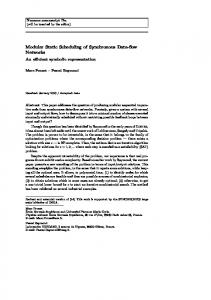
We have built a preliminary implementation of the SDF modular code generation described above in the Ptolemy II framework [3]. The implementation uses a specialized class to describe composite SDF actors for which DSSF profiles can be generated. These profiles are captured in Java, and can be loaded when the composite actor is used within another composite. For debugging and documentation purposes, the tool also generates in the GraphViz format DOT (http://www.graphviz.org/) the graphs produced by the unfolding and clustering steps. Using our tool, we can, for instance, generate automatically a profile for the Ptolemy II model depicted in Figure 13. This model captures the SDF model given in Figure 3 of [4]. Actor A2 is a composite actor designed so as to consume 2 tokens on each of its input ports and produce 2 tokens on each of its output ports every time it fires. It uses for this the DownSample and UpSample internal actors: DownSample consumes 2 tokens at its input and produces 1 token at its output; UpSample consumes 1 token at its input and produces 2 tokens at its output. Actors A1 and A3 are homogeneous. The SampleDelay actor models an initial token in the queue from A2 to A3. All other queues are initially empty. The DAG produced by unfolding and the clustering produced by GBDC on the top-level Ptolemy model is shown to the left of Figure 14. This graph is automatically generated by DOT from the textual output automatically generated by our tool. The two replicas of A1 are denoted A1 1 0 and A1 2 0, respectively, and similarly for A2 and A3. Two clusters are generated, giving rise to the profile shown to the right of the figure. Notice that the profile contains only two nodes, despite the fact that the Ptolemy model contains 9 actors overall.

17

Figure 13: A hierarchical SDF model in Ptolemy II.

Cluster_0 A1_1_0 Cluster_1 A1_2_0

1

A3_1_0

1

port A2_1_0

1 A3_2_0

port4 2

1

f1 1

1

1 f2

port2 1 port3 2

Figure 14: Clustering (left) and DSSF profile (right) of the model of Figure 13.

18

10

Conclusions and Perspectives

Hierarchical SDF models are not compositional: a composite SDF actor cannot be represented as an atomic SDF actor without loss of information that can lead to deadlocks. Extensions such as CSDF are not compositional either. In this paper we introduced DSSF profiles as a compositional representation of composite actors and showed how this representation can be used for modular code generation. In particular, we provided algorithms for automatic synthesis of DSSF profiles of composite actors given DSSF profiles of their sub-actors. This allows to handle hierarchical models of arbitrary depth. We showed that different tradeoffs can be explored when synthesizing profiles, in terms of modularity (keeping the size of the generated DSSF profile minimal) versus reusability (preserving information necessary to avoid deadlocks) as well as algorithmic complexity. We provided a heuristic DAG clustering method that has polynomial complexity and ensures maximal reusability. In the future, we plan to examine how other DAG clustering algorithms could be used in the SDF context. This includes the clustering algorithm proposed in [8], which may produce overlapping clusters, with nodes shared among multiple clusters. This algorithm is interesting because it guarantees an upper bound on the number of generated clusters, namely, n + 1, where n is the number of outputs in the DAG. Overlapping clusters result in complications during profile generation that need to be resolved. Profile generation could also be improved to generate more compact profiles. For example, for the composite actor of Figure 15 our method currently generates the profile shown to the bottom-left of the figure. P.f1 corresponds to firing A; A; B, P.f2 to firing A; B and P.f3 to firing A; B. Since P.f2 and P.f3 are identical, we could represent them as one, instead of two firing functions, and obtain the profile shown to the bottom-right of the figure, which is more compact. This could be the result of some re-folding operation that is to be defined. P 1

3

4

A

2

1 B

1 P.f1

2

2

1

P.f2

1

1 1 1

1 P.f1

1

P.f3

2

2

1

1

P.f2

1

1

Figure 15: Re-folding. We would also like to study possible applications of DSSF to contexts other than modular code generation, for instance, compositional performance analysis, such as throughput or latency computation. Finally, we plan to study possible extensions to dynamic data flow models.

Acknowledgments We would like to thank J¨ orn Janneck and Maarten Wiggers for interesting discussions.

References [1] S. Bhattacharyya, E. Lee, and P. Murthy. Software Synthesis from Dataflow Graphs. Kluwer, 1996. 19

[2] G. Bilsen, M. Engels, R. Lauwereins, and J. A. Peperstraete. Cyclo-static data flow. In IEEE Int. Conf. ASSP, pages 3255–3258, May 1995. [3] J. Eker, J. Janneck, E. Lee, J. Liu, X. Liu, J. Ludvig, S. Neuendorffer, S. Sachs, and Y. Xiong. Taming heterogeneity – the Ptolemy approach. Proc. IEEE, 91(1), January 2003. [4] J. Falk, J. Keinert, C. Haubelt, J. Teich, and S. Bhattacharyya. A generalized static data flow clustering algorithm for mpsoc scheduling of multimedia applications. In Embedded Software – EMSOFT’08, pages 189–198. ACM, 2008. [5] M.C.W. Geilen. Reduction of Synchronous Dataflow Graphs. In Design Automation Conference, DAC 2009. ACM, 2009. [6] E.A. Lee and D.G. Messerschmitt. Static scheduling of synchronous data flow programs for digital signal processing. IEEE Trans. Comput., 36(1):24–35, 1987. [7] R. Lublinerman, C. Szegedy, and S. Tripakis. Modular code generation from synchronous block diagrams: modularity vs. code size. In Principles of Programming Languages – POPL’09, pages 78–89. ACM, January 2009. [8] R. Lublinerman and S. Tripakis. Modularity vs. reusability: code generation from synchronous block diagrams. In Design, Automation and Test in Europe – DATE’08, pages 1504–1509. ACM, March 2008. [9] J.L. Pino, S.S. Bhattacharyya, and E.A. Lee. A Hierarchical Multiprocessor Scheduling Framework for Synchronous Dataflow Graphs. Technical Report UCB/ERL M95/36, EECS Department, University of California, Berkeley, 1995. [10] S. Sriram and S. Bhattacharyya. Embedded Multiprocessors: Scheduling and Synchronization. Marcel Dekker, Inc., 2000.

20