In particular, we consider the fundamental dictionary problem on set data, where the task is to construct a data structure to represent a set S of n items out of a ...
Compressed Data Structures: Dictionaries and Data-Aware Measures? Ankur Gupta, Wing-Kai Hon, Rahul Shah, and Jeffrey Scott Vitter?? {agupta,wkhon,rahul,jsv}@cs.purdue.edu Department of Computer Sciences, Purdue University, West Lafayette, IN 47907–2066, USA Abstract. We propose measures for compressed data structures, in which space usage is measured in a data-aware manner. In particular, we consider the fundamental dictionary problem on set data, where the task is to construct a data structure to represent a set S of n items out of a universe U = {0, . . . , u − 1} and support various queries on S. We use a well-known data-aware measure for set data called gap to bound the space of our data structures. We describe a novel dictionary structure taking gap+O(n log(u/n)/ log n)+O(n log log(u/n)) bits. Under the RAM model, our dictionary supports membership, rank, select, and predecessor queries in nearly optimal time, matching the time bound of Andersson and Thorup’s predecessor structure [AT00], while simultaneously improving upon their space usage. Our dictionary structure uses exactly gap bits in the leading term (i.e., the constant factor is 1) and answers queries in near-optimal time. When seen from the worst case perspective, we present the first O(n log(u/n))-bit dictionary structure which supports these queries in nearoptimal time under RAM model. We also build a dictionary which requires the same space and supports membership, select, and partial rank queries even more quickly in O(log log n) time. To the best of our knowledge, this is the first of a kind result which achieves data-aware space usage and retains near-optimal time.
1
Introduction
The proliferation of data is suffocating our abilities to manage information. The information content in many cases is relatively low, and with proper representation, there is much potential to save space. The new trend of data structure design considers time and space efficiency together: The ultimate goal is to build structures that operate in the optimal (or nearly so) time bound, while requiring the minimum amount of space, tuned for the particular input data. Ideally, the space required for a structure should be defined with respect to the Kolmogorov complexity of the data upon which the structure is built, as it is the space of the smallest program that can generate the input data. Unfortunately, it is undecidable for arbitrary input, making it an inconvenient measure for practical use. On the other hand, there may be simple space measures that are sensitive enough to capture the information in the input data set. Consider set data, which represent a subset S of n items from a universe U = {0, . . . , u − 1}. In many natural examples of set data, items are not purely randomly distributed among the universe. Examples include IP addresses, UPC barcodes, and ISBN numbers. These types of data sets are clustered and items are close to one another. The gap measure [BMNM+ 93] (described formally in Section 2.2) has been used extensively as a reasonable space measure in the context of inverted indexes [WMB99]. ?
??
Support was provided in part by the Army Research Office through grant DAAD20–03–1–0321 and by the National Science Foundation through research grant IIS–0415097. Support was provided in part by an IBM Faculty Research Grant.
The gap measure counts the space required to encode the distances between successive items and is usually much less than the information-theoretic (combinatorial) lower � u bound dlog n e ≈ n log(u/n) bits.1 (This bound is known as the information-theoretic minimum � because it is the minimum number of bits needed to differentiate between the nu possible subsets of n items�out of a universe of size u.) A gap-style encoding can be much smaller than dlog nu e bits for many of the data sets above, since it exploits short distances between items. In this paper, we present compressed representations for both fully indexable dictionaries (FID) and indexable dictionaries (ID), improving the space required by previous results without sacrificing near-optimal query time. In particular, under the unit-cost RAM model, we develop a fully indexable dictionary (FID)—a data structure supporting rank and select queries—of size gap +O(n log(u/n)/ log n) +O(n log log(u/n)) bits, while supporting rank in time matching Andersson and Thorup’s (nearly-optimal) predecessor structure [AT00] and select even faster in O(log log n) time. For typical parameter values (namely when n = o(u)), our fully indexable dictionary is asymptotically equal to gap space (with� a constant of 1) and is strictly less than the information-theoretic minimum dlog nu e bits. To our knowledge, this result is the first of its kind. Even when considered from a worst-case perspective, our data structures are the first to take O(n log(u/n)) bits with nearoptimal query time. We also develop an indexable dictionary (ID)—a data structure supporting partial rank and select queries—in the same number of bits that supports each query even faster in O(log log n) time. This result is the first to operate with gap-style bounds in space with time sublogarithmic in terms of the number of items stored. Moreover, our data structures are useful in practice; we have a practical implementation and we discuss algorithmic engineering and experimental results in a companion � paper [GHSV05]. Our preliminary results show that gap is about 40−60% u of dlog n e for many practical data sets.
1.1
Comparisons to Previous Work
Previously, Jacobson [Jac89], Munro [Mun96], Brodnik et al. [BM99], Pagh [Pag99], and Raman et al. [RRR02] develop dictionaries that support constant-time queries. The best among these are the ID (supporting partial rank and select) and the FID (supporting rank and select) by Raman et al.�[RRR02], �� which both support constantu time queries, and respectively require only log + o(n) + O(log log u) bits and n �� � u log n + O(u log log u/ log u) + O(log log u) bits. These results seem quite strong, as the constant factor associated with the information-theoretic minimum term is 1; unfortunately, the space is not bounded in a data-aware manner. Recent work by Grossi and Sadakane [GS06] achieves an FID with constant-time queries that requires gap + O(u log log u/ log u) bits of space. Still, these FID structures do not work well when n � u, as the o(u) term will be much � (even exponentially) larger than u the information-theoretic minimum term dlog n e, dwarfing any savings we want to achieve. Consider a typical example of maintaining a dictionary for � IP lookup, storing u 17 32 2 IP addresses out of a universe of size 2 . In this case, dlog n e is roughly 345,661 1
Throughout the paper, we assume the base of the logarithm is 2.
(about 218 ) bits while their o(u) term is roughly 6.71 × 10⁸ (about 229 ) bits—several � orders of magnitude larger than the information-theoretic minimum dlog nu e bits. Blandford and Blelloch [BB04] recently propose an interesting scheme that allows easy transformation of any FID implemented with O(n) pointers into another that requires O(gap) + O(uα log u) bits for any α < 1.2 After the transformation, query time is a factor of 1/α slower than the original dictionary. A fundamental aspect of a dictionary’s search capabilities is captured by the predecessor problem, since dictionaries that (implicitly) solve the predecessor problem require fundamentally more space and time than those that do not. Precisely, the predecessor query determines the largest item in S smaller than the query. Beame and Fich [BF99] describe a data structure that takes O(n2 log u) bits of space so that membership and predecessor queries can be solved in BF (u, n) = p O(min{(log log u)/(log log log u), (log n)/(log log n)}) time. They also show that this bound is tight as long as we have only O(nO(1) log u) bits available.3 Andersson and Thorup [AT00] provide a transformation to Beame and Fich’s data structure, improving the space to O(n log u) bits and making the data structure dynamic using exponential search trees. However, the query time increases to )! (s log log u log n log n . , · log log n, log log n + AT (u, n) = O min log log n log log log u log log u Since rank and select can be used to answer predecessor queries, we improve Andersson and Thorup’s structure in terms of space without sacrificing query time. In the worst case, our fully indexable dictionary compares favorably with both Raman et al. [RRR02] and Blandford and Blelloch [BB04]. With respect to the former, though we cannot support O(1)-time queries, we have eliminated the problematic o(u) space term. Our query time—which is AT (u, n)—is already close to the optimal BF (u, n). When comparing with [BB04], we note that their method can be tuned by some of the techniques developed in our paper to achieve (1 + �)gap bits of space. However, this increases their search time by a multiplicative factor of 1/�. In addition, they require either complex RAM operations or a decoding table that requires (potentially) much more space. For our indexable dictionary, when compared with Raman et al.’s ID structure [RRR02], we pay a small price in the lookup time in exchange for achieving space bounds in terms of gap, which may be significant in practice.
2
Dictionaries and Data Aware Measures
Let S = hs1 , . . . , sn i be an ordered set of n items from a universe U = {0, 1, . . . , u − 1} of size u; that is, i < j implies si < sj . We want to represent S in a succinct form so that we can also perform basic dictionary queries in its compressed representation. We define dictionaries more formally in Section 2.1. In Section 2.2 we describe two measures for representing the set S, motivating these as reasonable measures for 2 3
They only claim O(n log((u + n)/n)) + O(uα log u) bits in their paper. It is this result which necessitates Raman et al.’s FID [RRR02] o(u) space term, since constant-time rank and select queries imply constant-time predecessor queries as well.
analyzing the space required by a dictionary. We further show strong relationships between these measures in Section 2.3.
2.1
The Dictionary Problem
The dictionary problem appears as a fundamental black box in a number of applications used to offer fast access (for some queries, even constant-time access) to the data. Some examples include suffix arrays and IP lookup tries. In particular, dictionaries are key building blocks in encoding the Burrows-Wheeler transform (BWT) of a text succinctly and supporting fast decoding. Our interest is to exploit the great potential for a functional but compressed dictionary data structure. In some applications, dictionaries are the bottleneck, both in terms of space and query time. We describe some fundamental queries on set data. Here, a ∈ U and 1 ≤ i ≤ n. We define member(S, a), rank(S, a), select(S, i), prank(S, a), and pred(S, a) below. rank(S, a) = {si |si ≤ a} select(S, i) = si
member(S, a) = 1 if a ∈ S, 0 otherwise prank(S, a) = rank(S, a) if a ∈ S, −1 otherwise pred(S, a) = max{si |si ≤ a}
Definition 1. An indexable dictionary (ID) represents a subset S ⊆ U and supports the queries prank(S, a) and select(S, i). A fully indexable dictionary (FID) represents a subset S ⊆ U and supports the queries rank(S, a) and select(S, i). Fully indexable dictionaries can solve predecessor queries, and so they immediately find application in rich problem areas as IP lookup structures [CDG99], compressed text indexing [GGV03], and suffix arrays [GV00]. Sometimes, an item si is associated with a piece of satellite data di and an operation to lookup si returns the satellite data di . Note that this lookup can be supported by using rank and select operations.
2.2
The gap and trie Measures
One well-known method for representing the set S is gap encoding [BMNM+ 93], which is often used in compressing inverted indexes. (We refer the reader to [WMB99] for a detailed treatment of the various applications of this method, as well as a source for further references.) Consider the gaps between consecutive items in S, where the ith gap gi is equal to si − si−1 . We can now represent the set S as the stream of gaps G = g1 , . . . , gn , where g1 = s1 , along with the value n. The stream G of gaps can be stored using variable length encoding based on their size. Suppose we could store each gi in dlog(gi + 1)e bits. Then, the total space, which we call the gap measure, is gap(S) =
n X
dlog(gi + 1)e
i=1
bits. Note that a representation of S in gap(S) bits is not decodable, since we need to mark the separation between successive items. One popular technique to “mark” these separators is by using a prefix code such as the δ code [Eli75]. In δ coding, we represent each gi in dlog(gi +1)e+2 dlogdlog(gi + 1)ee bits, where the first dlogdlog(gi + 1)ee bits
are the unary encoding of the number dlogdlog(gi + 1)ee, the next dlogdlog(gi + 1)ee bits are the binary representation of the number dlog(gi +1)e, and the final dlog(gi +1)e bits are the binary representation of gi . With proper schemes, we can represent the stream of gaps G = g1 , g2 , ..., gn by concatenating the encoding of each gi such that G is uniquely decodable. We refer to these extra bitsPof overhead beyond gap(S) as the decoding overhead Z(S). For δ coding, Z(S) = 2 i dlogdlog(gi + 1)ee bits. By Jensen’s inequality,4 gap(S) is maximized when all gaps gi are the same. In this case, gap(S) would require roughly n log(u/n) bits, since each of the n gaps would be of size u/n. Z(S) is also maximized in this case for δ coding. Hence, Z(S) is roughly 2n log log(u/n) bits. Other prefix codes, such as the γ code [Eli75] and some combination of Huffman and fixed-length coding result in a somewhat different Z(S). In this paper, we use the δ encoding scheme, and denote the bit representation of S using this encoding by GAP(S). The size of GAP(S) is |GAP(S)| = gap(S) + Z(S) bits. Another method for compression of S is the prefix omission method (POM) [KS02], which is generally used to represent bitstrings of arbitrary length. Consider the bitstrings sorted lexicographically. We can represent each bitstring with respect to the previous bitstring by omitting the common prefix of the two. To compress S by POM, we think of each item of S as its log u-length bit representation. The POM for S can also be seen as a subtree (of n leaves) of the complete binary tree on u leaves (which is a trie). Each root-to-leaf path in this trie defines an item s in S. For x, y ∈ S, let x y denote the bitstring formed by omitting the common prefix of x and y from the bit representation of x. To represent S by POM, we generate the stream L = l1 , l2 , . . . , ln , where l1 is the bit representation of s1 in log u bits and li = si si−1 . Let |li | denote the number of bits in li . Thus, the cost of this representation, which we call the trie measure, is trie(S) =
n X
|li | = |s1 | +
i=1
n X
|si si−1 |,
i=2
which equals the number of edges in the trie. Similar to the gap measure, the above representation with trie(S) bits is not decodable as each string li is P of variable length. Hence, we need some extra bits Z 0 (S) for decoding, which takes 2 i dlog |li |e bits in the case of δ encoding. Similarly, we use TRIE(S) to denote the bit representation of S using POM, which takes |TRIE(S)| = trie(S) + Z 0 (S) bits of space. Let S + a denote the set in which the positive integer a is added (modulo u) to each item of S. Thus, the set S + a is {(s1 + a) mod u, (s2 + a) mod u, . . . , (st + a) mod u}. We define the shifted trie measure strie(S) = mina {trie(S + a)}, which corresponds to the number of bits needed to compress S by POM under the ‘best shift’. We denote STRIE(S) to be the corresponding TRIE(S + a).
2.3
Relationship Between gap, trie and strie
In this section, we show a strong relationship between the gap, trie and strie measures. For any item si , dlog(gi + 1)e is always smaller than |li |, but |li | could be much larger. 4
For a concave function f and x1 + x2 + · · · + xk = x,
i
f (xi ) is maximized when xi = x/k.
For example, when si−1 = 2k − 1 and si = 2k , |li | = k even though dlog(gi + 1)e = 1. We show that this scenario cannot occur too frequently and prove that trie(S) ≤ 2gap(S). However, by applying a ‘random shift’, such cases are nearly eliminated. In the following lemma, we bound trie(S) more tightly using this intuition. We omit the proof of Lemma 1 due to space constraints, but it follows from a counting argument for the number of bits required for a particular gap gi under all possible shifts. Lemma 1. The trie measure on the set S + a, trie(S + a), is at most gap(S) + 2n − 2 bits on average over all values of a ∈ [1, u]. Thus the shifted trie measure, strie(S), is at most gap(S) + 2n − 2. Note that |li | is bounded on average by dlog(gi + 1)e + 2 bits. Since the decoding overP head is d2 log |li |e with the δ code, we can bound the total overhead 2 i dlog |li |e by 2n log log(u/n) bits using Jensen’s inequality. Thus, the space requirement |STRIE(S)| is at most strie(S) + 2n log log(u/n) + log u bits.
0
4
1 0
1
1
8
3
1
1
8
13
0
0
0
1
0
1
0
1
1
15
12
1
4
0
13 0
9
1
0
9
12
15
1001
4
0100
8
001
0
9
12
13
101
0
11
15
Fig. 1. The left hand side shows a binary search tree built on the items 1, 4, 8, 9, 12, 13, and 15. Beneath that is its pre-order layout on disk, where the arrows represent pointers to the right subtree. The right hand side shows the trie built on the same items. Beneath that is the corresponding layout on disk, but each item s is encoded with respect to anc(s). For instance, 8 is encoded in the layout on the right as 0, since anc(8) = 9 differs from it by a single bit.
Binary Searchable Dictionary Representation
Despite all the development on the POM model, the trie encoding of S does not support time-efficient queries as we would like. Klein and Shapira [KS02] use the trie encoding to search in compressed dictionaries, but their searching algorithm essentially consists of a linear scan of the items in the dictionary and takes at least Ω(n) time. Most algorithms using gap encoding also need a linear scan. In this section, we build a binary searchable data structure BSD, which resolves rank and select queries in O(log n) time. We show that the space required by this structure is gap bits plus low-order terms. In fact, the main point of this section is in showing that a binarysearchable representation requires about the same number of bits as simple linear encoding schemes. Also, BSD is our main building block and will be used later in this paper to support fast lookup in our FID and ID dictionary structures. The BSD structure encodes a pre-order traversal of a balanced binary search tree T built on the n items of S. In Figure 1, the pre-order traversal for the set S is 9, 4, 1, 8, 13, 12, and 15. The key point is that instead of storing each item si explicitly in log u bits, we encode an item with respect to an ancestor anc(si ), defined as follows. Let Ai be the set of all the ancestors of si in the binary search tree T . Then, anc(si ) =
x ∈ Ai such that lcp(si , x) is maximized over all ancestors in Ai . We represent si by si anc(si ) using log u − |lcp(si , anc(si ))| bits, similar to our trie encoding. Now we define the BSD(S) encoding. We use a recursive layout to describe the pre-order traversal of the binary search tree of n items. Let the subsets SL = hs1 , s2 , ..., sdn/2e−1 i and SR = hsdn/2e+1 , ..., sn i represent the left and right subtrees of the sdn/2e th item. In general, we define Si,j = hsi , si+1 , ...sj i. Let anc(sdn/2e ) = 0. For BSD(S), let |BSD(S)| denote the number of bits needed to encode BSD(S). Then, we define the BSD encoding as BSD(S) = hsdn/2e anc(sdn/2e ); |BSD(SL )|; BSD(SL ); BSD(SR )i. Note that sdn/2e anc(sdn/2e ) is a variable-length string, which is stored using δ coding. The term |BSD(SL )| constitutes additional overhead but is needed in order to jump to the right half of the set while searching. It turns out that BSD requires nearly the same space as does the TRIE encoding. Next, we describe how rank and select functions are supported in O(log n) time using BSD(S) and analyze its space usage. In Sections 4 and 5, we use BSD(S) as a black box on O(log n) items and achieve O(log log n) time; in order to do so, we must be able to decode a δ-coded item (or bitstring) in O(1) time in the RAM model. We assume that the word size of the machine is at least log u bits, and that we are allowed to perform addition, subtraction, multiplication, and bitshift operations in O(1) time. We also assume that we can calculate the position of the leftmost 1 of a subword x of log log u bits in O(1) time. (This task is equivalent to calculating dlog(x + 1)e when the word x is seen as an integer.) We can also easily encode and decode the operator using bitshifts and additions. These assumptions are sufficient to allow O(1) decoding time. If this model is not applicable, we can simulate the decoding by explicitly storing the decoding result of every possible log log u-bit number in a table with log u entries. Note that this table takes O(log u log log log u) bits, which is negligible overhead. In order to support rank and select, we just need to store the single value n (in log n bits) at the beginning of the BSD to indicate how many items are stored within the structure. Since our structure is a well-defined balanced binary tree, at any node x with nx items, we know that the size of our left subtree contains dnx /2e − 1 items, and our right subtree contains nx − dnx /2e items. Hence, we can compute rank and select based upon this information. More precisely, given BSD(S), rank(S, a) and select(S, i) can be computed in O(log n) time by calling the recursive functions rrank(BSD(S), a, 0, u, n) and rselect(BSD(S), i, 0, u, n) as detailed below. function rrank(B, a, `, r, n) function rselect(B, i, `, r, n) if (n = 0) return 0; x ← root(BSD(S)); x ← root(B); z ← decode(x, `, r); z ← decode(x, `, r); if (i = dn/2e) return z; if (z = a) return dn/2e + 1; else if (i > dn/2e) else if (z < a) return rselect(BSD(SR ), i − dn/2e, z, r, n − dn/2e); return dn/2e + rrank(BSD(SR ), a, z, r, n − dn/2e); else return rselect(BSD(SL ), i, `, z, dn/2e − 1); else return rrank(BSD(SL ), a, `, z, dn/2e − 1);
In the pseudocode, the function root(B) returns the first encoded string in B (i.e., root(B) = si anc(si )), and the function decode(x, `, r) returns the item si that corresponds to the root of B. The latter function can be computed by first
determining anc(si ), which is one of ` or r based on the first bit of root(B). Then, si = (anc(si ) div 2y ) × 2y + root(B), where y = |root(B)|. We denote rank(S, a) and select(S, i) functions for BSD(S) by BSD rank (B, a) and BSD select(B, i) where B is a pointer (of log u bits) to BSD(S). We shall use this notation in Sections 4 and 5. We now bound the space of our BSD(S) representation. Lemma 2. The BSD(S) representation requires at most trie(S) + O(n log log(u/n)) bits and supports rank and select in O(log n) time. Proof. (sketch) The space of BSD(S) can be divided into three parts: (i) the space for all si anc(si ); (ii) their decoding overhead; and (iii) the space to encode all |BSD(SL )|, used to jump to the right half of the encoding. The space for (i) can be shown to be equal to the number of edges in the trie, which is exactly trie(S). For (ii), the overhead is analogous to Z(S) and we can bound it by O(n log log(u/n)) using Jensen’s inequality. For (iii), it can be bounded by a path recursion sum and shown to be O(n log log(u/n) + n) bits. t u The above lemma suggests that BSD(S +a) requires min a {|BSD(S +a)|} bits, which is at most gap(S) + O(n log log(u/n)) bits by Lemma 1. For the rest of the paper, we assume the BSD representation for S is based on its best shift. We obtain the following theorem, which is used in constructing our data structures in Sections 4 and 5. Theorem 1 (BSD). The BSD(S) representation is a fully indexable dictionary (FID) requires gap(S)+O(n log log(u/n)) bits and supports rank and select in O(log n) time.
4
The Fully Indexable Dictionary Structure
We describe our structure in a bottom-up way. At the bottom level, we store a BSD dictionary for every log2 n items from set S, each of which can resolve a rank or select query in O(log log n) time. We also store B.f irst rank along with each BSD B, where B.f irst rank is the rank in S of its first item in B. We also keep an array P [1..dn/ log2 ne], where P [i] stores a pointer to the ith BSD structure, which stores the items s(i−1) log2 n+1 , . . . , si log2 n . This structure alone is sufficient to support select. In order to support rank, let Sˆ = {si |i mod (log2 n) = 1} be the set of smallest items from each BSD. We build an instance of Andersson and Thorup’s predecessor ˆ called R. To support rank, we use a lookup dictionary L from structure [AT00] on S, Section 2.1 built on Sˆ as keys with pointers to the corresponding BSD as satellite data. We denote the process of looking up the satellite data associated with s ∈ Sˆ by L.lookup(s). Then, rank and select can be solved as follows. function rank(S, a) s ← pred(R, a); B ← L.lookup(s); return B.f irst rank + BSD rank (B, a);
function select(S, i) j ← di/(log 2 n)e; B ← P [j]; return BSD select (B, i − B.f irst rank + 1);
We obtain the main theorem below, along with a worst-case analysis, since gap and O(n log log(u/n)) are bounded by O(n log(u/n)).
Theorem 2. Given a set S of n items from a universe [1, u], we implement an FID in gap(S) + O(n log(u/n)/ log n) + O(n log log(u/n)) bits so that rank takes AT (u, n) time and select takes O(log log n) time. In the worst case, our data structure takes O(n log(u/n)) bits of space with the same time bounds.
5
The Indexable Dictionary Structure
In this section, we build upon our earlier approach and partition S into lower level BSD structures, each of size at most log3 n. We use a top level ‘distributor’ structure to access the correct BSD while answering a rank query. If the query item is not present in S, our top level distributor may not return any associated BSD; therefore, we cannot support rank or predecessor queries. Our top level distributor takes O(log log n) time to return the correct BSD, since our partitioning scheme is somewhat more complex than that of our FID. Since searching in an O(log n) size BSD structure is similarly bounded, we can support partial rank and select queries in O(log log n) time. To bound the overhead space required by our top level distributor, we limit the number of partitions to at most O(n log log n/ log 3 n) to match the same second-order term as in our FID. Next, we outline our top level distributor structure, which is similar to the van Emde Boas (VEB) tree [vEBKZ77]. With this distributor structure, for any x ∈ U , we can either report that x ∈ / S or obtain the BSD that might contain x. Our distributor structure is a recursive structure analogous to a VEB tree. Instead of having O(log log u) levels of recursion as in the case for a VEB tree, our distributor only has h = 3 log log n levels. At the top level (Level 1), we have a single distributor (with parameter p = 0 to be explained shortly) to distribute all items in S. For level i = 1 to h−1, a Level i distributor with parameter p connects to some Level i+1 distributors, which are then used to distribute the items recursively; the parameter p indicates that all the items in the distributor share the same first p bits. At the bottom level (Level h), a Level h distributor directs the items to their designated BSD structures. More precisely, for i = 1 to h − 1, a Level i distributor with parameter p = pi works as follows: 1. Partition the items into groups according to the first pi + log u/2i bits. 2. For each group with more than log3 n items (which we call a dense group), the items are passed to a Level i + 1 distributor with parameter p = pi + log u/2i . 3. For all items not in a dense group, they are grouped together. (a) If the number of items is at most log3 n, the items are passed to a Level h distributor with parameter p = pi . (b) Else, the items are passed to a Level i + 1 distributor with parameter p = pi . Theorem 3. Given a set S of n items from a universe [1, u], we implement an indexable dictionary (ID) in gap(S) + O(n log(u/n)/ log n) + O(n log log(u/n)) bits supporting partial rank and select queries in O(log log n) time.
6
Conclusions
In this paper, we have formalized and developed measures for analyzing the space needed to store set data. These measures provide a framework for further investiga-
tion of compressed data structuring techniques. We have achieved a fully indexable dictionary that operates in near-optimal time (AT (u, n)) to support rank, select, and predecessor queries, while taking just gap + O(n log(u/n)/ log n) + O(n log log(u/n)) bits of storage. Our result improves a number of existing compressed data structures [AT00,RRR02,BB04] by reducing space usage, while maintaining nearly-optimal time bounds. Our gap term has a constant of 1, which is extremely important when considering space efficiency. Equally important are � the properties of the the other space terms—if n = o(u), they amount to o(log nu ) bits. Also, our dictionary is the first that achieves O(n log(u/n)) bits of space, without sacrificing the query times. We also provide an indexable dictionary which operates in the same space and supports queries in O(log log n) time.
References [AT00]
A. Andersson and M. Thorup. Tight(er) worst-case bounds on dynamic searching and priority queues. In Proceedings of the ACM Symposium on Theory of Computing, 2000. [BB04] D. Blandford and G. Blelloch. Compact representations of ordered sets. In Proceedings of the ACM-SIAM Symposium on Discrete Algorithms, 2004. [BF99] P. Beame and F. Fich. Optimal bounds for the predecessor problem. In Proceedings of the ACM Symposium on Theory of Computing, 1999. [BM99] A. Brodnik and I. Munro. Membership in constant time and almost-minimum space. SIAM Journal on Computing, 28(5):1627–1640, October 1999. [BMNM+ 93] T. C. Bell, A. Moffat, C. G. Nevill-Manning, I. H. Witten, and J. Zobel. Data compression in full-text retrieval systems. Journal of the American Society for Information Science, 44(9):508– 531, 1993. [CDG99] P. Crescenzi, L. Dardini, and R. Grossi. Ip address lookup made fast and simple. In Proceedings of the European Symposium on Algorithms, pages 65–76, 1999. [Eli75] P. Elias. Universal codeword sets and representations of the integers. IEEE Transactions on Information Theory, IT-21:194–203, 1975. [GGV03] R. Grossi, A. Gupta, and J. S. Vitter. High-order entropy-compressed text indexes. In Proceedings of the ACM-SIAM Symposium on Discrete Algorithms, January 2003. [GHSV05] A. Gupta, W. K. Hon, R. Shah, and J. S. Vitter. Compressed dictionaries: Space measures, data sets and experiments, 2005. In preparation. [GS06] Roberto Grossi and Kunihiko Sadakane. Squeezing succinct data structures into entropy bounds. In Proceedings of the ACM-SIAM Symposium on Discrete Algorithms. To appear, 2006. [GV00] R. Grossi and J. S. Vitter. Compressed suffix arrays and suffix trees with applications to text indexing and string matching. In SIAM Journal on Computing, 35(2):378–407. A shorter version appeared in the ACM Symposium on Theory of Computing, May 2000. [Jac89] G. Jacobson. Succinct static data structures. Technical Report CMU-CS-89-112, Department of Computer Science, Carnegie-Mellon University, January 1989. [KS02] S. T. Klein and D. Shapira. Searching in compressed dictionaries. In Proceedings of the IEEE Data Compression Conference, 2002. [Mun96] J. I. Munro. Tables. Foundations of Software Technology and Theoretical Computer Science, 16:37–42, 1996. [Pag99] R. Pagh. Low redundancy in static dictionaries with O(1) worst case lookup time. In Proceedings of the International Colloquium on Automata, Languages, and Programming, 1999. [RRR02] R. Raman, V. Raman, and S. S. Rao. Succinct indexable dictionaries with applications to encoding k-ary trees and multisets. In Proceedings of the ACM-SIAM Symposium on Discrete Algorithms, pages 233–242, 2002. [vEBKZ77] P. van Emde Boas, R. Kaas, and E. Zijlstra. Design and implementation of an efficient priority queue. Math. Systems Theory, 10:99–127, 1977. [WMB99] I. H. Witten, A. Moffat, and T. C. Bell. Managing Gigabytes: Compressing and Indexing Documents and Images. Morgan Kaufmann Publishers, Los Altos, CA, 2nd edition, 1999.