COMPRESSIVE SAMPLING FOR ENERGY SPECTRUM ESTIMATION

c 2014 Society for Industrial and Applied Mathematics

SIAM J. SCI. COMPUT. Vol. xx, No. x, pp. x–x

COMPRESSIVE SAMPLING FOR ENERGY SPECTRUM ESTIMATION OF TURBULENT FLOWS∗

arXiv:1404.5653v1 [physics.flu-dyn] 22 Apr 2014

GUDMUNDUR F. ADALSTEINSSON† AND NICHOLAS K.-R. KEVLAHAN‡ Abstract. Recent results from compressive sampling (CS) have demonstrated that accurate reconstruction of sparse signals often requires far fewer samples than suggested by the classical Nyquist–Shannon sampling theorem. Typically, signal reconstruction errors are measured in the ℓ2 norm and the signal is assumed to be sparse, compressible or having a prior distribution. Our spectrum estimation by sparse optimization (SpESO) method uses prior information about isotropic homogeneous turbulent flows with power law energy spectra and applies the methods of CS to 1-D and 2-D turbulence signals to estimate their energy spectra with small logarithmic errors. SpESO is distinct from existing energy spectrum estimation methods which are based on sparse support of the signal in Fourier space. SpESO approximates energy spectra with an order of magnitude fewer samples than needed with Shannon sampling. Our results demonstrate that SpESO performs much better than lumped orthogonal matching pursuit (LOMP), and as well or better than wavelet-based best M -term or M/2-term methods, even though these methods require complete sampling of the signal before compression. Key words. Compressive sampling, turbulence, energy spectrum, wavelets, optimization. AMS subject classifications. 76F05, 65F22, 65T60.

1. Introduction. Sampling and storage of signals becomes challenging for high wavenumber or high dimensional signals if the Nyquist–Shannon sampling theorem is followed strictly. The theory of compressive sampling (CS) provides a rigorous framework to accurately reconstruct a signal from a few non-adaptive (random) projections, provided it is sufficiently sparse or compressible in some basis [7, 15, 9]. Since statistically homogeneous turbulent signals are not known for their high compressibility, the use of CS for turbulence is on the edge of applicability. In addition, turbulence researchers are often more interested in reconstructing Fourier energy spectra from spatial measurements and spectrum estimation is not a well-developed area of CS. d Consider the discrete signal u ∈ Rn of length N = nd in d dimensions. The traditional fixed-rate sampling, hereafter referred to Shannon sampling, of u is inefficient if the coefficients u ˆ of u in an orthogonal basis are sufficiently compressible. Shannon sampling is especially wasteful if we are interested only in a particular low dimensional property of the signal, such as the one-dimensional energy spectrum of a two- or three-dimensional data set. This paper focuses on the reconstruction of energy spectra of homogeneous isotropic turbulent flows from a minimal number of samples. A turbulent flow is characterized by a non-dimensional number, the Reynolds number Re, which is the ratio of inertial terms to viscous terms in the Navier–Stokes equations governing the flow. Flows become turbulent when Re exceeds a certain threshold (typically ∼ 103 ) and industrial and natural turbulent flows have very large Reynolds numbers (∼ 105 –1012 ). The minimum length scale of a turbulent flow, the Kolmogorov scale η, decreases with increasing Reynolds number Re like η ∝ Re−3/4 [17], and the number of spatial samples required by the sampling theorem in d dimensions is N ∝ η −d . Therefore, the † School of Computational Science and Engineering, McMaster University, Hamilton, ON L8S 4K1, Canada ‡ Department of Mathematics and Statistics, McMaster University, Hamilton, ON L8S 4K1, Canada ∗ Submitted to the SIAM Journal on Scientific Computing on April 22, 2014.

1

2

G. F. ADALSTEINSSON AND N. K.-R. KEVLAHAN

total number of samples needed to characterize a turbulent flow increases very quickly with Reynolds number: like Re9/4 in three dimensions and Re3/2 in two dimensions. Thus, straightforward application of Shannon sampling requires huge amounts of regularly sampled data (∼ 1011 –1027 ) to estimate the complete one-dimensional energy spectrum of a three-dimensional turbulent flow. However, because the range in wavenumber space of the one-dimensional energy spectrum of u is proportional to η −1 ∝ Re3/4 , there is definitely room for improved sampling strategies. Even for one-dimensional signals, such as hot-wire measurements, it should be possible to accurately characterize the energy spectrum using fewer samples than required for the usual Shannon sampling. In order to accurately estimate the one-dimensional energy spectra of signals with a very large and continuous range of active length scales, we propose a new method that uses a priori information about the signal, such as the structure and scaling of wavelet coefficients, isotropy, and power law behaviour of the energy spectrum. We show that our method is able to approximate energy spectra with an order of magnitude fewer samples than needed with Shannon sampling. We introduce notation and give a brief introduction to CS in section 2 before we define our problem and introduce two measurement matrix types used in our experiments. In section 3.2 we introduce the relevant wavelet transforms and their application to turbulence, and finally present our SpESO algorithm for estimating energy spectra. Section 5 verifies the method by applying it to a set of representative test cases: 1-D hot-wire turbulence data, 1-D synthetic power-law data, 2-D numerical simulation turbulence data and 2-D synthetic power-law signals. In related work, variants of CS have been developed to estimate spectra and other properties of signals, but in different contexts which do not apply in our case. In [13] linear functions of signals were estimated by fast operators. Energy spectra, however, are nonlinear functions of signals. Sparse and locally supported 2-D spectra were estimated in [32], but turbulence is not sparse in Fourier space. Similarly, [19, 2] put some sparsity constraints on their power spectrum estimation. Bands of power spectra are estimated on a linear scale from non-uniform samples in [20]. In [1] the 2-D spectrum itself is sampled and approximated to reduce computational time in spectroscopy. General nonlinear optimization problems for CS are considered in [4]. However, the iterative algorithm proposed is impractical in our case as it requires expensive high dimensional gradients to be computed at each iteration. 2. Compressive sampling for large signals. In this paper we assume that the turbulent flow is provided as a single component of a turbulent velocity vector field as a discrete sequence u ∈ RN . Mathematically, of course, the flow is more accurately described as velocity (or vorticity) vector field of velocity defined on a three-dimensional spatial domain. However, assuming the flow is band-limited in wavenumber, the Nyquist–Shannon sampling theorem allows us to represent it as sequence of discrete values. The measurement matrices discussed later are discrete approximations of linear operators in continuous space. We represent two-dimensional signals of dimension n × n as vectors of length N = n2 . We first decompose u as a linear combination of vectors in a basis Φ ∈ RN ×N , X u ˆi φi , (2.1) u = Φˆ u= i

where u ˆ are the expansion coefficients and φi are the basis vectors. A signal u is said to be B-sparse in basis Φ if | supp(ˆ u)| = B < N , where | · | denotes cardinality and

COMPRESSIVE SAMPLING FOR SPECTRUM ESTIMATION

3

supp(x) = {i : xi 6= 0} is the support. The signal u is called compressible in the basis Φ if it has ordered coefficients |ˆ u|(1) ≥ · · · ≥ |ˆ u|(N ) that satisfy the inequality |ˆ u|(n) ≤ Cn−s for s > 0 and a constant C [8]. The best B-term approximation in an orthonormal basis, fB , is an approximation with all but the B largest terms of u ˆ zero. Many signals are highly compressible in a wavelet basis [14] since wavelet basis functions are self-similar and are localized in both position and scale. If the signal is compressible then the error in the best B-term approximation is kfB − f k = O(B −s+1/2 ). The central idea of CS, see e.g. [7, 15, 9, 10], is that a few linear non-adaptive (e.g. random) measurements of a signal are sufficient to accurately reconstruct a signal if that signal is compressible in some basis. Note that the measurement scheme (e.g. random samples) and the sparsity system (e.g. a wavelet basis) must be mutually incoherent in the sense of having a sufficiently small maximum inner product between the basis vectors of the measurement scheme and the sparsity system. Let A ∈ RM×N be a measurement matrix , let g ∈ RM be the compressed samples, and assume M < N . The measurement scheme is defined by the under-determined system g = Au.

(2.2)

In a slightly different form, with Ψ = AΦ which we call the CS-matrix, we have g = Ψˆ u,

(2.3)

where u ˆ is assumed to be B-sparse in the basis Φ. Under this framework, the minimization problem [10] ˆ ℓ1 u ˆ⋆ = arg min khk

ˆ = g, s.t. Ψh

(2.4)

N ˆ h∈R

is proved to accurately approximate, or exactly reconstruct, the original signal, provided some basic conditions on the structure of Ψ and the compressibility of the signal are satisfied. (A star superscript, u⋆ , denotes approximation.) This method is called basis pursuit and can be solved via convex optimization. Unfortunately, turbulent signals are not compressible enough in wavelet bases for basis pursuit to give meaningful results, especially in the high wavenumber range of the spectrum. Reconstruction methods which are significantly faster than the basis pursuit method for (2.4) include so-called greedy methods. A popular greedy method is iterative orthogonal matching pursuit (OMP) [30]. Our estimation algorithm relies heavily on a multi-level modification of OMP called QOMOMP, see section 3.2. OMP can be generalized easily to estimate more than one coefficient of the signal at a time [33]. The experiments in section 5 use Lumped OMP (LOMP) as a comparison to our SpESO method, where the sparsity B0 is fixed and L0 coefficients are estimated in each iteration, requiring a total of B0 /L0 iterations. The initial CS literature was largely concerned with full random measurement matrices A, which require O(N M ) operations to apply to a vector. Many CS decoding methods require frequent application of A and its transpose. For very large signals the matrix–vector multiplications are very memory and CPU intensive [6], so a full random matrix is not practical. In our method we consider two matrices with fast matrix-free transforms requiring at most O(N log N ) operations and O(N ) memory to apply.

4

G. F. ADALSTEINSSON AND N. K.-R. KEVLAHAN

The first matrix is intended for measurements of 1-D time-dependent signals— such as hot-wire measurements—without requiring the whole signal for every compressed sample: a random finite impulse response (FIR) filter [31]. Let the filter coefficients h be compactly supported with support size K. We can then write A = RΓ F ∗ ΣF,

(2.5)

where Σ = diag(F h) is a diagonal matrix where the diagonal elements are the Fourier transform of h, and F is the Fourier transform matrix. Here RΓ restricts the result to an evenly distributed set Γ of length M . This definition of A assumes periodicity, but our implementation zero pads the signal before the convolution to account for nonperiodic boundary conditions. For a downsampling fraction δ0 and with 1/δ0 ∈ N, the number samples is M = ⌈(N + K − 3)δ0 ⌉,

(2.6)

and the complexity is O(KM ). A random convolution and sub-sampling is a universal sampling strategy [28]. Consider now a full vector h and a diagonal matrix Σ = diag(h) which randomizes the phase, i.e. hk = eiθk , where θk are i.i.d. uniformly distributed on (0, 2π) such that F ∗ Σ ∈ RN . We can again write A = RΓ F ∗ ΣF,

(2.7)

where R restricts the result to a random set Γ. The complexity of this approach is O(N log N ). Note that the random convolution matrix A has the property that its right pseudo-inverse is the transpose, AT (AAT )−1 = AT (i.e. AAT = I or A is right-orthogonal). We use this matrix (or measurement scheme) for analyzing 2-D data. 3. Energy spectrum estimation of turbulence data. 3.1. Problem formulation. Our problem is challenging because we seek to estimate the energy spectrum E(k) from measurements of u, rather than estimating u directly. This problem is challenging because the quantity to be estimated, E(k), is a nonlinear function of the quantity that is sampled, u. In addition, u is not sparse in Fourier space. Dropping the constant normalization factor, let us define E(k) as E(k) =

X

k≤|k′ | Λ(ˆ u⋆ω )} ⊲ locate large coefficients in Γj−1 Ω⋆ ← children(ω ⋆ ) ⊲ corresponding coefficients in Γj aΓcj ← 0 ⊲ coefficients outside Γj will not be selected ⊲ adjust elements of a with a large parent coefficient (in uˆ⋆ ) aΩ⋆ ← βaΩ⋆

a priori we know that wavelet coefficients are relatively large above a certain scale and, on average, the magnitude of wavelet coefficients decreases monotonically with decreasing scale. We call this method quasi-oracle multilevel orthogonal matching pursuit (QOMOMP), see Algorithm 1. QOMOMP will be used to efficiently solve the minimization problem (2.4), which is the key computational step of our energy spectrum estimation method. QOMOMP estimates all coefficients at levels less than a pre-defined coarsest level j < J0 . The “initial coefficient index set by oracle” defined by J0 is chosen such that almost all wavelet coefficients up to level J0 are large, approximately large enough to be included in the best M/2-term approximation. At each finer scale j ≥ J0 a pre-defined number of coefficients, Lj , is estimated. We will see later that the choice of the sequence L = {Lj } is a key factor determining the performance of the method. Discrete wavelet coefficients have a tree-like structure, where (in 1-D) the two child coefficients at a fine scale j are more likely to be large if their parent coefficient at the coarse scale j − 1 is large. To enforce this tree-like structure of the non-zero wavelet coefficients u ˆ⋆ we apply the function tree(a), see Algorithm 2, to modify the raw wavelet coefficients of the residual in the QOMOMP Algorithm 1. This is similar to the method used in [18], but enforces the tree structure less strictly. The tree algorithm 2 works as follows. Let Γj be the index set for level j and Ω be the current support of wavelet coefficients u ˆ⋆ at iteration j in QOMOMP. The index ⋆ set ω identifies those coefficients at the coarse level j − 1 above a threshold defined by Λ. Then, Ω⋆ = children(ω ⋆ ) are the child coefficients at level j of the significant parent coefficients ω ∗ at level j − 1. Finally, the tree function scales the residuals a in Ω⋆ by a constant, aΩ⋆ ← βaΩ⋆ . If β > 1 this makes the residuals corresponding

COMPRESSIVE SAMPLING FOR SPECTRUM ESTIMATION

7

2

10

1

CPU time [s]

10

0

10

QOMOMP N/M ≈ 16 QOMOMP N/M ≈ 4 C·N C · N log3 N

-1

10

3

10

4

10

5

10

6

10

N

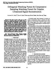
Fig. 1. Computational cost of QOMOMP (measured by CPU time) versus signal length N , showing mean curves and standard deviation bars of 16 random simulations. The number of samples is a fixed ratio of N , either N/M = 16 or N/M = 4, and the measurement matrix is a filter of length K = 284. The number of coefficients L is a fixed ratio of N such that the sparsity is B/M ≈ 0.79.

to children at scale j of significant wavelet coefficients at scale j − 1 more likely to be selected as the Lj largest coefficients. If β = 1 tree(a) does nothing, while in the limit β → ∞ it exactly enforces a tree structure. Isotropy of the signal is not of concern in 1-D. In 2-D, however, the diagonal wavelet coefficients, denoted by k = 3 in (3.6), of a best B-term approximation of an isotropic signal become a smaller proportion of the total for a particular level as the scale decreases. To account for this we let the operator | · |> Lj in QOMOMP in 2-D choose the coefficients such that the diagonal ones are a ratio qj of the total for level j. The least squares problem in Algorithm 1 is solved using an iterative method for the normal equation. The relative tolerances are fixed, except for the last level where we decrease the tolerance for higher accuracy. Numerical verification of the computational cost of QOMOMP, Figure 1, confirms that it scales linearly with the signal size N for typical parameters. Intermediate and final tolerances are set to ǫi = 2 × 10−2 and ǫf = 3.3 × 10−6 , respectively. Now, let us return to the energy spectrum estimation problem stated in (3.3). Let L0 be the initial sequence of the number of non-zero coefficients at each level for QOMOMP and let the index set J specify those levels for which we want to optimize the sequence L. With u⋆ an estimate provided by QOMOMP we iteratively approximate min k log(EAT Au ) − log(EAT Au⋆ )kwj , Lj

∀j ∈ J

(3.7)

where the weights wj are constant with support in the range 2j−1 < k ≤ 2j . We put the constraints Lj ≤ Lj−1 in 1-D and Lj ≤ 2Lj−1 in 2-D for j ∈ J . We call this low dimensional optimization spectrum estimation by sparse optimization 1 (SpESO). Since the computation of u⋆ is expensive and the optimization function is non-smooth, we do not solve (3.7) exactly. Instead, we search amongst values uniformly distributed on a log scale and narrow the search after each iteration. From the linear dependency of QOMOMP on N and the implementation of SpESO, we estimate the overall computational complexity of SpESO to be O(N |J |). 1 The

code for SpESO with QOMOMP is available at github.com as SpESO.

8

G. F. ADALSTEINSSON AND N. K.-R. KEVLAHAN

Our experiments show that decoupling the matrix used in SpESO from the one used in QOMOMP improves the convergence properties. By that, we mean that the ˜ giving a set of measurement matrix is split horizontally into two parts A and A, ˜ measurements g = Au and g˜ = Au. For QOMOMP we use Ψ = AΦ and g and for ˜ and vice versa. The two estimated spectra are then combined SpESO we use A˜T A, proportionally to their relative errors. A simplistic argument for the decoupling is that since QOMOMP minimizes the error Au⋆ − g to a small or zero value regardless of L, then the difference between AT Au and AT Au⋆ will be small and (3.7) will not converge to any meaningful minimum. By using two separate matrices this problem disappears and results in a better correlation between a good choice of L and a low energy spectrum error. The downside is that QOMOMP only uses half of the measurements for each estimation. 4. Analysis of the performance of SpESO for ideal signals. We now analyze mathematically the convergence and accuracy of SpESO. Let us consider the restricted isometry property (RIP) of the CS matrices that determines the accuracy of reconstructions. The restricted isometry constant of a matrix Ψ is the smallest number δB such that [11, 5] (1 − δB )kxk ≤ kΨxk ≤ (1 + δB )kxk

(4.1)

holds for all x at most√B-sparse. If the OMP algorithm is applied with a matrix Ψ satisfying δB+1 < 1/( B + 1), then it recovers a B-sparse signal exactly [34]. The proof is mainly concerned with showing that at each iteration the index chosen is in the true support T . Given the true support at the final iteration, the reconstruction is trivial. Assume T is the true support of the best B-term approximation uB . In the case of a perfect oracle where Ω = T in QOMOMP, the solution to the final least squares problem is ˆT c ), u ˆ⋆T = Ψ+ u = Ψ+ ˆ T + ΨT c u T Ψˆ T (ΨT u

(4.2)

∗ where Ψ+ ˆ⋆T = T is a pseudo-inverse. With ΨT ΨT non-singular (δB < 1) we get u + ˆT c . Therefore, the error is u ˆ T + ΨT ΨT c u

kˆ uT − u ˆ⋆T k = kΨ+ ˆT c k T ΨT c u

(4.3)

or, with Φ orthonormal u−u ˆ B k2 + ˆT c k2 ≤ kˆ ku − u⋆ k2 = kˆ uT c k2 + kΨ+ T ΨT c u

1 kΨ(ˆ u−u ˆB )k2 1 − δB

(4.4)

(the inequality follows from RIP [24]). For a compressible signal u, the error depends on the best B-term approximation error kˆ uT c k = ku − uB k and the least squares error term, which depends on the RIP of the matrix Ψ. Given u is B-sparse (u = uB ), the error vanishes. Now consider our QOMOMP method in a very simple 1-D setting to obtain some quantitative performance estimates. Let QOMOMP be applied to a signal u with a power law energy spectrum k −α , where 0 < α ≤ 2n + 1 is limited by the number of vanishing moments n of the wavelet used in the sparsity system. The variance of the wavelet coefficients at each level then scales like Var(dˆji )i ∼ 2−jα [27]. Assuming u is a Fourier synthetic signal like those considered in section 5, then dˆji for each level is well

COMPRESSIVE SAMPLING FOR SPECTRUM ESTIMATION

9

approximated as i.i.d. with a Gaussian distribution and zero mean. If ΩJ0 = ∪j