Original Articles
© Schattauer 2009
Computation of a Probabilistic Statistical Shape Model in a Maximum-a-posteriori Framework H. Hufnagel1, 2; X. Pennec1; J. Ehrhardt2; N. Ayache1; H. Handels2 1INRIA Asclepios
2Department
Project, Sophia Antipolis, France; of Medical Informatics, University Medical Center Hamburg-Eppendorf, Hamburg, Germany
Keywords
Statistical shape model, registration, ICP, EMICP, correspondence problem
Summary
Objectives: When analyzing shapes and shape variabilities, the first step is bringing those shapes into correspondence. This is a fundamental problem even when solved by manually determining exact correspondences such as landmarks.We developed a method to represent a mean shape and a variability model for a training data set based on probabilistic correspondence computed between the observations. Methods: First, the observations are matched on each other with an affine transformation found by the Expectation-Maximization Iterative-Closest-Points (EM-ICP) registration.We then propose a maximum-a-posteriori (MAP) framework in order to compute the statistical shape model (SSM) parameters which result in an optimal adaptation of the model to the observations. The optimization of the MAP explanation is realized with respect to the Correspondence to: Heike Hufnagel Department of Medical Informatics University Center Hamburg Eppendorf Martinistr. 52, S 14 20246 Hamburg Germany E-mail:
[email protected]
1. Introduction The representation and analysis of 3D shape variabilities is of importance in different medical imaging problems, for example when dealing with 4D image data as breathing lungs [1, 2] or beating hearts [3], when computing an anatomical variability atlas as e.g.
observation parameters and the generative model parameters in a global criterion and leads to very efficient and closed-form solutions for (almost) all parameters. Results: We compared our probabilistic SSM to a SSM based on one-to-one correspondences and the PCA (classical SSM). Experiments on synthetic data served to test the performances on non-convex shapes (15 training shapes) which have proved difficult in terms of proper correspondence determination. We then computed the SSMs for real putamen data (21 training shapes). The evaluation was done by measuring the generalization ability as well as the specificity of both SSMs and showed that especially shape detail differences are better modeled by the probabilistic SSM (Hausdorff distance in generalization ability ˜ 25% smaller). Conclusions: The experimental outcome shows the efficiency and advantages of the new approach as the probabilistic SSM performs better in modeling shape details and differences.
Methods Inf Med 2009; 48: ■–■ doi: 10.3414/ME9228 prepublished: ■■■
shown in [4] or when solving segmentation problems. One of the central difficulties of analyzing different organ shapes in a statistical manner is the identification of correspondences between the points of the shapes. As the manual identification of landmarks is not a feasible option in 3D, several preprocessing techniques were developed to
automatically find exact one-to-one correspondences between surfaces which are represented by meshes [5–8]. A popular method is to optimize for correspondences and registration transformation as does the Iterative Closest Points (ICP) algorithm [9] for point clouds. More elaborate methods directly combine the search of correspondences and of the SSM for a given training set as proposed in [10, 11] or the Minimum Description Length (MDL) approach to statistical shape modeling [12, 13]. The MDL is used to optimize the distribution of points on the surfaces of the observations in the training data set when determining the best SSM. For unstructured point sets, the MDL approach is not suited to compute a SSM because it needs explicit surface information. Another interesting approach proposes an entropy-based criterion to find shape correspondences, but requires implicit surface representations [14]. Other approaches combine the search for correspondences with shape-based classification [15, 16] or with shape analysis [17], however, these methods are not easily adaptable to multiple observations of unstructured point sets as they either depend on underlying surface information or fix the number of points representing the surface. The approach in [18] for unstructured point sets focuses only on the mean shape. In all cases, enforcing exact correspondences for surfaces represented by unstructured point sets leads to variability modes that not only represent the organ shape variations but also artificial variations whose importance is linked to the local sampling of the surface points. Therefore, we believe that a method for shape analysis should better rely on probabilistic point locations as presented with the EM-ICP registration in [19]. Based on this, we advanced the probabilistic concept of [20] to compute a probabilistic SSM for unstructured point sets. Methods Inf Med 4/2009
1
2
H. Hufnagel et al.: Computation of a Probabilistic Statistical Shape Model in a Maximum-a-posteriori Framework
Fig. 1
2. Methods We argue that when segmenting anatomical structures in noisy image data, the extracted surface points only represent probable surface locations. Based on this, it is very difficult to find the true shape surface. In our probabilistic approach, we propose a maximum-aposteriori framework in order to compute the model parameters which result in an optimal adaptation of the model to the observations in a global unique criterion. The optimization of the MAP explanation is realized with respect to the generative model parameters and all observation parameters and leads to very effi-
cient and closed-form solutions for (almost) all parameters without the need of one-to-one correspondences as is usually required by the PCA. We then compute the SSM which best fits the given data set by optimizing the global criterion iteratively with respect to all model and all observation parameters.
2.1 Statistical Shape Model Built on Correspondence Probabilities In the process of computing the SSM, we distinguish strictly between model parameters and observation parameters. The generative
SSM is explicitly defined by four model parameters: – ● Mean shape M ∈ R3m parameterized by Nm points mj ∈ R3. ● Variation modes vp consisting of Nm 3D vectors vpj . ● Associated standard deviation λp which describes the impact of the variation modes. ● Number n of variation modes. – Using the generative model Θ = {M, vp, λp, n} of a given structure, the shape variations of that structure can be generated by Mk = – M+
ωkpvp with ωkp ∈ R being the defor-
mation coefficients. The shape variations along the modes follow a Gaussian probability distribution with variance λp: p(Mk | Θ) = p(Ωk | Θ) = Πp p(ωkp | Θ) = (1)
Fig. 2
Synthetic training data set featuring banana shapes. a) Observation examples; b) probabilistic SSM; c) classical SSM. Mean shapes (middle) and mean shapes deformed with respect to the first variation mode. Left: – → M – 3λv1 and right: – → M + 3λv1. d) Result example of leaveone-out experiment. Left: SSM built on one-to-one correspondences. Right: SSM built on probabilistic correspondences. The deformed mean shapes are dark grey while the obsrevation is colored in light grey.
Methods Inf Med 4/2009
with Ωk ∈ Rn being a vector consisting of the deformation coefficients ωkp associated with shape variation Mk. In order to account for the unknown position and orientate on of the model in space, we introduce the random (uniform) rigid or affine transformation Tk. A model point mj can then be deformed and placed by Tk omkj = . Finally, we specify the sampling of the model surface: Each sampling (e.g. observation) point si is modeled as a Gaussian measurement of a (transformed) model point mkj . The probability of the observation p (ski | mkj , Tk) knowing the originating model point mkj is given by the equation you can see in Figure 1.As we do not know the originating model point for each ski , the probability of a given observation point ski is described by a mixture of Gaussians and the probability for the whole scene Sk becomes: p(Sk | Μ, Tk) =
(2)
We summarize the observation parameters as Qk = {Tk, Ωk}. Notice that the correspondences are hidden parameters that do not belong to the observation parameters of interest. © Schattauer 2009
H. Hufnagel et al.: Computation of a Probabilistic Statistical Shape Model in a Maximum-a-posteriori Framework
2.2 Derivation of the Global Criterion Using a MAP Approach When building the SSM, we use a training data set containing N observations Sk ∈ R3Nk, and we are interested in the parameters linked to the observations Q = {Qk} as well as the unknown model parameters Θ. In order to determine all parameters of interest, we optimize a MAP on Q and Θ. (3) . As p(Sk) does not depend on Θ and p(Θ) is assumed to be uniform, the global criterion integrating our unified framework is the following: C(Q, Θ) =
(4)
Starting from the initial model parameters Θ, we then fit the model to each of the observations. Next, we fix the observation parameters Qk and update the model parameters. This is iterated until convergence.
2.3 Evaluation Methods In order to asses the quality of the probabilistic SSM, we compare its performance to a ‘classical’ SSM as e.g. used in [8]. The classical SSM is based on exact correspondences found by an iterative closest points (ICP) registration and its variation modes are determined by a classical principal component analysis (PCA). In the following, we first explain the measures we use to quantify the performance of an SSM and state which distance measures we use. Next, we describe the design of the experiments.
2.3.1 Performance Measures The first term describes the maximum likelihood (ML) criterion ( Eq. 2) whereas the second term is the prior on the deformation coefficients ωkp as described in Equation 1. Dropping the constants, our criterion simplifies to C(Q, Θ) ~ Ck(Qk, Ω) with C(Qk, Θ) = . (5)
This equation is the heart of the unified framework for the model computation and its fitting to observations. By optimizing it alternately with respect to the operands in Qk = {Tk, Ωk} we are able to determine all parameters we are interested in. In a first step, all observations are aligned with the initial mean shape by estimating the Tk using the EM-ICP. In order to robustify, we used a multi-scaling scheme concerning the variance σ2, that is we start with a great σstart in order to align positions, rotation and sizes. The variance is then reduced in each iteration to cover for shape details. This approach seems to be quite robust to the choice of initial mean shape [21]. © Schattauer 2009
For both SSMs, we compute two performance measures, the generalization ability and the specificity as proposed in [22]. The generalization ability indicates how well a SSM is able to match new unknown shapes. This is important e.g. when using the SSM to segmentation problems. The generalization ability is tested in a series of leave-oneout experiments. We analyze how closely the SSM matches an unknown observation. The SSM is first aligned with the new observation. Then, the optimal deformation coefficients are determined and used to deform the aligned SSM in order to optimize the matching. Finally, the distance of the deformed SSM to the left-out observation is measured. For aligning the probabilistic SSM using the EMICP registration, similar parameters as for the SSM computation were used, that is, the registration was not optimized for each unknown observation. The specificity indicates how well the modeled variability represents the variability found in the training data set. For estimating the specificity, a high number (in our case 500) of random shapes have to be generated which are uniformly distributed with their variances equal to the variance or eigenvalues of the respective SSM. Then, the distances of the random shapes M idef to the most similar observation S idef in the training data set is measured.
2.3.2 Distance Measures There are several options to compute a similarity measure between two shapes (source and target). As in our case the shape surfaces are represented by point clouds, we compute the distances based on point coordinates. Hence, we define the distance d from an observation Sk to the deformed mean shape Mdef with Nm points mj as d(Sk, Mdef ) =
where
mki = arg minmj || ski – mj ||. This distance measure is not symmetric, hence, we also compute d(Mdef, Sk) = where skj = arg min . In addition, we compute the maximum distance dmax (Sk , Mdef ) as the maximal minimal distance found from Sk to Mdef for || ski – mki || with mki = arg minmj || ski – mj || and respectively dmax(Mdef, Sk). The Hausdorff distance is then max(dmax(Mdef , Sk), dmax(Sk , Mdef ). Furthermore, we determine the mean difference between the pairs d(Mdef , Sk) and d(Sk , Mdef ) as a measure of symmetry. As symmetric distance measures we define the averaged mean distance dmean(Sk , Mdef ) = and the averaged maximum distance dav – max (Sk , Mdef ) = . The symmetric measures are especially useful for estimating the specifity as the deformed model has to be compared to all observations in the training data set in the same reference frame.
2.3.3 Design of Experiments We conducted two sets of experiments, one on synthetic data and one on real data. Shapes with non-convex or even non-starshaped surfaces are a challenge for the computation of a SSM as the automatic determination of correspondences is difficult.As we later want to use the SSM for segmenting structures like the kidney or the acetabulum, Methods Inf Med 4/2009
3
4
H. Hufnagel et al.: Computation of a Probabilistic Statistical Shape Model in a Maximum-a-posteriori Framework Table 1 Banana shape results. Shape distances found in generalization experiments (six leave-oneout tests) and in specificity test with probabilistic SSM approach and with the SSM-ICP approach. The distances and associated standard deviations are given in mm. Generalization ability
Classical SSM
Probabilistic SSM
d(Mdef , Sk ) in mm
18.82 ± 3.49
19.43 ± 5.46
d(Sk, d(Mdef )) in mm
30.37 ± 15.75
20.28 ± 5.14
dmax(Mdef , Sk ) in mm
48.84 ± 18.47
63.62 ± 32.07
dmax(Sk , Mdef ) in mm
84.31 ± 53.41
49.57 ± 12.83
average | d(Mdef , Sk) – d(Sk , Mdef ) | in mm
11.56 ± 12.6
1.31 ± 1.06
18.87 ± 9.73
30.74 ± 2.78
Specificity dmean (Sk , Mdef ) in mm
Fig. 3
Real training data set featuring the putamen. a) Observation examples; b/c) probabilistic SSM; d/e) classical SSM. Mean shapes (middle) and mean shapes deformed with respect to the first (b, d) and second (c, e) variation mode. Left: – → M – 3λv1, 2 and – → right: M – 3λv1,2 . The regions in circles mark shape details which are represented by the probabilistic SSM and which are not modeled by the classical SSM.
Methods Inf Med 4/2009
an analysis of a SSM method regarding nonconvex shapes is of great interest. In order to test how the probabilistic SSM and the classical SSM deal with non-convex shapes, we generated a synthetic data set containing 15 observations shaped like bananas (see Fig. 2a). In order to obtain meaningful results, the variability in the training data set is high: The curvature of the banana as well as the size, thickness and orientation in space changes from observation to observation. The number of points range from minimum 386 to maximum 642. The average smallest distance between the points is 29.3 mm. The experiments served to prove that the probabilistic SSM is suited better for training data sets containing nonconvex shapes. Our real data set consisted of N = 21 left segmented putamen observations (approximately 20 mm × 20 mm × 40 mm) which are represented by minimum 994 and maximum 1673 points ( Fig. 3a). The MR images (255 × 255 × 105 voxels of size 0.94 mm × 0.94 mm × 1.50 mm) as well as the manual segmentations were kindly provided by the Hôpital La Pitié-Salpêtrière, Paris, France. The data was collected in the framework of a study on hand dystonia. The computation of a SSM for the putamen data might be useful either for segmentation purposes or for an analysis of the shape variability in patient and control groups. We again evaluated the quality of a probabilistic SSM and a classical SSM.
3. Results 3.1 Synthetic Data Results We computed a classical and a probabilistic SSM for the banana training data set; for the results see Figures 2b and 2c. For the probabilistic SSM, the following parameters were chosen: σstart = 15 –100 mm (dependent on the observation shape), reduction factor = 0.9, 10 iterations (EM-ICP multi-scaling) with five SSM iterations. For the classical SSM using the ICP and the PCA, we iterated the ICP 50 times. Most of the parameter values were found in an heuristic way. The tests for the generalization ability for the banana SSMs were performed on six different left-out observations. The estimation of the specificity was performed on 500 random shapes. The results are represented in Table 1. © Schattauer 2009
H. Hufnagel et al.: Computation of a Probabilistic Statistical Shape Model in a Maximum-a-posteriori Framework
The distance values for the probabilistic SSM in general are lower than those of the classical SSM in the generalization ability experiment. Especially the maximum distances differ with 84.31 mm for the classical SSM and 63.63 mm for the probabilistic SSM. Also the difference between the values of |d(Mdef , Sk) – d(Sk , Mdef )| is considerably large with 11.56 mm for the classical SSM and 1.31 mm for the probabilistic SSM. The specificity tests show lower distance values for the classical SSM.
3.2 Real Data Results For our SSM, the following parameters were chosen: σstart = 4 mm, reduction factor = 0.85, 10 iterations (EM-ICP multi-scaling) with five SSM iterations. For the ICP+PCA SSM, we iterated the ICP 50 times. Most of the parameter values were found in an heuristic way. The results are shown in Figures 3b/c for the probabilistic SSM and in Figures 3d/e for the classical SSM. The results of the testing series for the generalization ability and the specificity for both our SSM and the ICP+PCA SSM on putamen data are depicted in Table 2. Regarding the generalization ability, we obtained an average mean distance of 0.610 mm for the classical SSM and an average mean distance of 0.447 mm for the probabilistic SSM. The average maximum distances read 4.288 mm for the classical SSM and 2.526 mm for the probabilistic SSM. These results concur with the images which show the first and second variation modes/eigenmodes for the probabilistic and classical SSM, here the deformations of the probabilistic SSM account for more details than those of the classical SSM 2. The specificity tests show similar distance values for the classical and the probabilistic SSM.
4. Discussion Especially the outcome for the values of |d(Mdef , Sk) – d(Sk , Mdef )| shows that the probabilistic SSM is able to capture for shape details which are lost for the classical SSM. Moreover, the Hausdorff distances in the gen© Schattauer 2009
Table 2 Putamen results. Shape distances found in generalization experiments (seven leave-one-out tests) and in specificity test with probabilistic SSM approach and with the SSM-ICP approach. The distances and associated standard deviations are given in mm.
Generalization ability
Classical SSM
Probabilistic SSM
dmean (Sk , Mdef ) in mm
0.610 ±0.089
0.447 ± 0.101
dav – max (Sk , Mdef ) in mm
4.388 ± 0.930
2.426 ± 0.712
0.515 ± 0.117
0.452 ± 0.020
Specificity dmean (Sk , Mdef ) in mm
eralization ability tests are more than smaller for the probabilistic SSM than for the classical SSM in the experiment on synthetic data. This is also illustrated in Figure 2d where the result of a rather extreme leave-one-out experiment is shown. The classical SSM adapts very well the corpus of the banana but fails to deform into its tip. The probabilistic SSM, however, is coming close to represent also the tip of the banana. This is due to the fact that the ICP only takes into account the closest point when searching for correspondence, thus, the points at the tip of the bananas are not necessarily involved in the registration process. The EM-ICP, however, evaluates the correspondence probability of all points, therefore, also the points at the tip are matched. For the same reason, the specificity values are better in the classical SSM as the standard deviations λp which were used for the random shape distributions are smaller in the classical SSM than in the probabilistic SSM. This is due to the fact that the classical SSM models less variability than the probabilistic SSM. Furthermore, in the test series on putamen data, our SSM achieved superior results in the generalization ability. Especially the reduced maximum distance (more than 40% smaller) illustrate the benefit of the new approach. In the figures displaying both SSMs it can be seen that the mean shapes of both approaches resemble, however, the first and second variation mode of the probabilistic SSM show more details than the first and second eigenmodes of the classical SSM. In conclusion, there are various shape details which are not captured very well by the ICP-SSM but can be modeled by the probabilistic SSM. This is an advantage when dealing with observations whose shapes differ significantly form those in the training data set or when the training data set contains two different shape classes.
Additionally, for segmenting unknown shapes of the same type, a well-modeled variability is of great importance. On the other hand, the classical SSM is easier to handle as the computation is straight forward and fast. For the probabilistic SSM, however, the practical convergence rate has to be investigated more carefully. For instance, a fast decrease of the multi-scale variance σ2 easily freezes the model in local minima and several parameter values are chosen heuristically in dependence of the number and distribution of points representing the observation shapes.
5. Conclusion We proposed a mathematically sound and unified framework for the computation of model parameters and observation parameters and succeeded in determining a closed form solution for optimizing the associated criterion alternately for all parameters. Experiments showed that our algorithm works well and leads to plausible results. It seems to be robust to different initial mean shape choices and is stable even for small numbers of observations. A good modeling of the variability is an important feature of a SSM, especially when it is employed to the segmentation of anatomical structures for radiotherapy or surgery planning where the precision must be high. We showed the efficiency of our approach compared with a SSM built by the traditional ICP and PCA for a non-convex and non-starshaped shape and found that the probabilistic SSM performs better in terms of generalization ability. From a theoretical point of view, a very powerful feature of our method is that we are optimizing a unique criterion. Thus, the conMethods Inf Med 4/2009
5
6
H. Hufnagel et al.: Computation of a Probabilistic Statistical Shape Model in a Maximum-a-posteriori Framework
vergence is ensured. Currently, we continue to evaluate the performance of the probabilistic SSM on different synthetic data such as nonspherical shapes which pose a problem for other well-established SSM methods as for example the otherwise effective MDL approach. Besides, we are working on an application of the probabilistic SSM on segmentation problems.
Acknowledgments The MR images as well as the segmentations of the putamen data were kindly provided by the Hôpital La Pitié-Salpêtrière, Paris, France. This work is supported by a grant from the German Research Foundation (DFG, HA2355/7-1).
References 1. Werner R, Ehrhardt J, Frenzel T, Säring D, Lu W, Low D, Handels H. Motion Artifact Reducing Reconstruction of 4D CT Image Data for the Analysis of Respiratory Dynamics. Methods Inf Med 2007; 46 (3): 254–260. 2. Handels H, Werner R, Frenzel T, Säring D, Lu W, Low D, Ehrhardt J. 4D Medical Image Computing and Visualization of Lung Tumor Mobility in Spatio-temporal CT Image Data. International Journal of Medical Informatics 2007; 76S: 433–439. 3. Säring D, Ehrhardt J, Stork A, Bansmann MP, Lund GK, Handels H. Computer-Assisted Analysis of 4D Cardiac MR Image Sequences after Myocardial Infarction. Methods Inf Med 2006; 45(4): 377–383. 4. Hacker S, Handels H. Framework for Representation and Visualization of 3D Shape Variations of
Methods Inf Med 4/2009
Organs in an Interactive Anatomical Atlas. Methods Inf Med 2009; 48 (3): 272–281. 5. Lorenz C, Krahnstoever N. Generation of PointBased 3D Statistical Shape Models for Anatomical Objects. Computer Vision and Image Understanding 2000; 77: 175–191. 6. Bookstein FL. Landmark methods for forms without landmarks: morphometrics in group differences in outline shapes. Medical Image Analysis 1996; 1: 225–243. 7. Styner M, Rajamani KT, Nolte LP, Zsemlye G, Székely G, Taylor CJ, Davies RH. Evaluation of 3D Correspondence Methods for Model Building. In: Proceedings of the International Conference on Information Processing in Medical Imaging 2003. pp 63–75. 8. Vos FM, de Bruin PW, Streeksa GI, Maas M, van Vliet LJ, Vossepoel AM. A statistical shape model without using landmarks. In: Proceedings of the International Conference of Pattern Recognition 2004. pp 714–717. 9. Besl PJ, McKay ND. A method for registration of 3D shapes. IEEE Transactions Pattern Analysis and Machine Intelligence 1992; 14: 239–256. 10. Zhao Z, Theo EK. A novel framework for automated 3D PDM construction using deformable models. Medical Imaging 2005; Proc of SPIE: Vol 5747: 303–314. 11. Chui H,Win L, Schultz R, Duncan JS, Rangarajan A. A unified non-rigid feature registration method for brain mapping. Medical Image Analysis 2003; 7: 113–130. 12. Davies RH, Twining CJ, Cootes TF. A Minimum Description Length Approach to Statistical Shape Modeling. IEEE Medical Imaging 2002; 21 (5): 525–537. 13. Heimann T, Wolf I, Williams T, Meinzer HP. 3D Active Shape Models Using Gradient Descent Optimization of Description Length. In: Proceedings of the International Conference of Pattern Recognition 2005. pp 566–577.
14. Cates J, Meyer M, Fletcher PT,Whitaker R. EntropyBased Particle Systems for Shape Correspondences. In: Proceedings of the Medical Image Computing and Computer Assisted Intervention 2006. pp 90–99. 15. Tsai A, Wells WM, Warfield SK, Willsky AS. An EM algorithm for shape classification based on level sets. Medical Image Analysis 2005; 9: 491–502. 16. Kodipaka S, Vemuri BC, Rangarajan A et al. Kernel Fisher discriminant for shape-based classification in epilepsy. Medical Image Analysis 2007; 11: 79–90. 17. Peter A, Rangarajan A. Shape Analysis Using the Fisher-Rao Riemannian Metric: Unifying Shape Representation and Deformation. IEEE Transactions on the International Symposium on Biomedical Imaging 2006. pp 1164–1167. 18. Chui H, Rangarajan A, Zhang J, Leonard C. Unsupervised learning of an atlas from unlabeled point-sets. IEEE Transactions Pattern Analysis and Machine Intelligence 2004; 26: 160–172. 19. Granger S, Pennec X. Multi-scale EM-ICP: A Fast and Robust Approach for Surface Registration. European Conference on Computer Vision 2002 in LNCS; Vol 2353: 418–432. 20. Hufnagel H, Pennec X, Ehrhardt J, Ayache N, Handels H. Generation of Statistical Shape Models with Probabilistic Point Correspondences and Expectation Maximization – Iterative Closest Point Algorithm. International Journal of Computer Assisted Radiology and Surgery 2008; 2(5): 265–273. 21. Hufnagel H, Pennec X, Ehrhardt J, Handels H, Ayache N. Shape Analysis Using a Point-Based Statistical Shape Model Built on Correspondence Probabilities. In: Proceedings of the Medical Image Computing and Computer Assisted Intervention 2007; Part 1:. pp 959–967. 22. Styner M, Gerig G, Lieberman J, Jones D, Weinberger D. Statistical shape analysis of neuroanatomical structures based on medial models. Medical Image Analysis 2003; 7: 207–220.
© Schattauer 2009