the search of correspondences and of the statistical shape model (SSM) for a given .... so the probability distribution model of its spatial location is the mixture.
Generation of a Statistical Shape Model with Probabilistic Point Correspondences and EM-ICP Heike Hufnagel1,2, Xavier Pennec1 , Jan Ehrhardt2, Nicholas Ayache1 und Heinz Handels2 1
2
Institut National de Recherche en Informatique et en Automatique (INRIA), Asclepios Project, 06902 Sophia Antipolis, France Department of Medical Informatics, University Medical Center Hamburg-Eppendorf, 20246 Hamburg, Germany
Abstract In this paper, we present a method to compute a statistical shape model based on shapes which are represented by unstructured point sets with arbitrary point numbers. A fundamental problem when computing statistical shape models is the determination of correspondences between the points of the shape observations of the training data set. In the absence of landmarks, exact correspondences can only be determined between continuous surfaces, not between unstructured point sets. To overcome this problem, we introduce correspondence probabilities instead of exact correspondences. The correspondence probabilities are found by aligning the observation shapes with the affine Expectation Maximization - Iterative Closest Points registration algorithm. In a second step, the correspondence probabilities are used as input to compute a mean shape (represented once again by an unstructured point set). Both steps are unified in a single optimization criterion which depends on the two parameters ’ registration transformation’ and ’mean shape’. In a last step, a variability model which best represent the variability in the training data set is computed. Experiments on synthetic data sets and real brain structure data sets are then designed to evaluate the performance of our algorithm. The method is compared to a statistical shape model built on exact correspondences. Results regarding the established measures ”generalization ability” and ”specificity” show the relevance of our approach.
1 Introduction One of the central difficulties of analyzing different organ shapes in a statistical manner is the identification of correspondences between the points of the shapes. As the manual identification of landmarks is not a feasible option in 3D, several preprocessing techniques were developed to automatically find exact one-to-one correspondences between surfaces which are represented by meshes [1,2,3,4]. A popular method is to optimize for correspondences and registration transformation as does the Iterative Closest Points (ICP) algorithm [5] for point clouds. More elaborate methods directly combine the search of correspondences and of the statistical shape model (SSM) for a given training set as proposed in [6,7] or the Minimum Description Length (MDL) approach to statistical shape modeling [8,9]. The MDL is used to optimize the distribution of points on the surfaces of the observations in the training data set when determining the best
SSM. For unstructured point sets, the MDL approach is not suited to compute a SSM because it needs an explicit surface information. Another interesting approach proposes an entropy based criterion to find shape correspondences, but requires implicit surface representations [10]. Other works combine the search for correspondences with shape based classification [11,12] or with shape analysis [13], however, these methods are not easily adaptable to multiple observations of unstructured point sets. The approach in [14] for unstructured point sets focuses only on the mean shape. The determination of correspondences between unstructured point sets is especially difficult when one shape features a certain structure detail and the other one does not, see Fig. 1. In all cases, enforcing exact correspondences for surfaces represented by unstructured point sets leads to variability modes that not only represent the organ shape variations but also artificial variations whose importance is linked to the local sampling of the surface points. To the best of our knowledge, no methods in the literature exist for the construction of a SSM based solely on unstructured point sets. We argue that when segmenting anatomical structures in image data with important noise, the extracted surface points only represent probable surface locations. Based on this, it is very difficult to find the true shape surface. Therefore we believe that a method for shape analysis should better rely only on the point locations and not on surface information. In this paper, we address the problem of building a SSM for shape observations represented by unstructured point sets with differing point numbers. In a first step, we determine correspondences probabilities between the shape model and all observations. We pursue a probabilistic concept by aligning the observations in a group-wise registration with the Expectation Maximization - Iterative Closest Point (EM-ICP) algorithm. The rigid EM-ICP was first introduced in 2002 by Granger and Pennec and proved to be robust, precise, and fast [15]. In this work, we generalize it to an affine transformation class. The SoftAssign algorithm [16] has a probabilistic formulation which is closely related but differs in that it gives the same role to the model and the observations. This is justified for a pair-wise registration but not for a group-wise model to observation registration. In a second step, we use the resulting correspondence probabilities as input to compute a mean shape for the training data set. We unify both steps under a unique global criterion which depends on the two parameters ’ registration transformation’ and ’mean shape’. The criterion is optimized iteratively with respect to both parameters. In a last step, we compute the variability model of the SSM. The modes of variation are computed using the standard Principal Component Analysis (PCA) on “virtual exact correspondences” which are determined by transforming the original points of the training shapes into ”virtual surface points” using the probabilistic correspondence information of the EM-ICP step. Finally, a comparison of our SSM and a SSM based on exact correspondences in terms of the established measures “generalization ability” and “specificity” is performed for evaluation. The remainder of this paper is organized as follows: The main steps of our algorithm the EM-ICP algorithm and the generation of the statistical shape model - are described in section 2. In section 3, the evaluation of the affine EM-ICP and the SSM is presented. Section 4 concludes the paper.
s2
s1
p1=0.05 p2=0.25
?
s3
p3=0.20
? s4
mj
p4=0.35
mj
? p5=0.15
s5
Figure 1. A correspondence problem: One shape features two bumps, the other only one. How can we determine correspondences between the two? Our approach establishes correspondence probabilities between all points representing the shape surfaces.
2 Methods and Material Our goal is to generate a SSM for a training data set of unstructured point sets which optimally represents the observations by a mean shape and a variability model. There are three steps on the way to compute the SSM: In the first step, we determine correspondence probabilities between the shapes. This is done by realizing a group-wise registration with the affine EM-ICP. In the second step, we define a criterion which depends on the correspondence probabilities, the registration transformations and the mean shape. The criterion is iteratively optimized with respect to all parameters in order to compute the mean shape. In the third and last step, we compute the variability with respect to the mean shape by transforming the original points of the training shapes into ”virtual surface points” using the probabilistic correspondence information of the EM-ICP step followed by a standard PCA. This chapter is organized as follows: The concept of the EM-ICP, our generalization to affine transformation classes and the role of the variance in the registration are explained in section 2.1. The subsequent generation of the SSM based on the correspondence probabilities is described in section 2.2. 2.1 The affine EM-ICP Algorithm The first step to compute a SSM is usually the determination of correspondences between the unstructured point set observations in the training data set. One of the first methods in the literature is the Iterative Closest Points (ICP) registration algorithm [5] which iteratively minimizes the sum of closest point distances between two shapes by deforming one of the shapes. However, we think that the ICP poses a problem for observations which feature distinctive shape detail differences as shown in Figure 1. We believe that it is advantageous to use correspondence probabilities instead of exact correspondences. The EM-ICP algorithm is a convenient method to find those. In the first part of this section, the concept of the EM-ICP is explained shortly for selfcompleteness (more details can be found in [15]). Then, we generalize the optimization of the transformation from rigid to affine transformation classes. Finally, we detail how the multi-scale scheme was adapted.
Correspondences Probabilities with the EM-ICP The EM-ICP algorithm determines the registration transformation T that best matches a model point set M ∈ (R 3 )Nm onto an observation point set S ∈ (R3 )Ns with Nm and Ns describing the number of points of the model and the observation respectively. The focus lies on the probability of an observation point si to be a measure of a transformed model point T ∗ mj . In that way, the point si is described as a displaced and noisy version of point mj . If the point si corresponds exactly to the model point mj , the measurement process can be modeled by a Gaussian probability distribution (see equation 1). p(si |mj , T ) =
1
1 exp(− (si − T ? mj )T .Σj−1 (si − T ? mj )) 2 (2π) |Σj | 1 2
3 2
(1)
where Σj represents the noise as the covariance of mj . However, the observation point si can in fact be a measure of any of the model points, so the probability distribution model of its spatial location is the mixture p(si |M, T ) =
Nm 1 X p(si |mj , T ). Nm j=1
(2)
Unfortunately, even if we assume that all scene point measurements are independent, no closed form solution exists for the maximization of p(S|M, T ). A solution is to model the unknown correspondences H ∈ RNs ×Nm as random hidden variables and to maximize the log-likelihood of the complete data distribution p(S, H|M, T ) efficiently using the EM algorithm. We denote E(Hij ) as the expectation of point si being an PN observation of point T ? mj (with the constraint j m E(Hij ) = 1) and find Ns X Nm 1 X E(log p(S, H|M, T )) = E(Hij ) log p(si |mj , T ). Nm i j
(3)
In the following, we assume uniform priors on H. In the Expectation-step, T is fixed and log p(S, H|M, T ) is estimated to compute E(H): exp(−µ(si , T ? mj )) P (Hij = 1) = E(Hij ) = P k exp(−µ(si , T ? mk ))
(4)
with µ(si , T ? mj ) = 12 (si − T ? mj )T .Σj−1 (si − T ? mj ). In the Maximization-step, E(H) is fixed and the estimated likelihood is maximized with respect to T . For this purpose, we do not have to take constants and normalizing factors into account, hence, the associated criterion CEM to be optimized takes the form as shown below: CEM (T, E) =
Ns X Nm X i
j
E(Hij )(si − T ? mj )T Σj−1 (si − T ? mj ).
(5)
Without loss of generality, we assume from now on a homogeneous and isotropic Gaussian noise with variance σ 2 in order to simplify the equations. The optimal transformation is then found by Ns X Nm 1 X Tˆ = argmin 2 E(Hij )ksi − T ? mj k2 . σ i j T
(6)
We see that the elements of E(H) serve as weighting factors. The solution of this leastsquares estimation for a rigid transformation T can be seen in [15]. Generalization to Affine Transformation We want to be able to analyse the variability of a training data set with respect to different transformations. Therefore, we generalize the EM-ICP to similarity and affine transformation classes. If we deal with an affine transformation Taf f it is Taf f ? mj = Amj + t with the transforming matrix A ∈ R3x3 and the translation vector t ∈ R3 . In order to find the best translation t we differentiate equation (5) with respect to t and obtain Nm Ns X ∂CEM (t) 1 X E(Hij )(si − Amj − t) = −2 2 ∂t σ i j m s m X X 1 X = −2 2 ( E(Hij ) − Ns t) si − A mj σ i i j
N
as
P Nm j
N
N
(7)
E(Hij ) = 1∀i. Thus, at the optimum we find Ns Ns Nm X 1 X 1 X E(Hij ). si − A mj tˆ = Ns i Ns j i
(8)
PN We see that tˆ aligns the barycentre s¯ = N1s i s si and the pseudo barycentre m ˜ = P Nm P Ns 1 mj i E(Hij ) of the two point clouds S and M . Using “barycentre” coorj Ns dinates s0 i = si − s¯ and m0 j = mj − m ˜ allows us to simplify the criterion into 0 CEM (T, E) =
Ns X Nm 1 X T T E(Hij )(s0 i s0 i − 2s0 i Am0 j + m0 j AT Am0 j ). σ2 i j
(9)
0 Next, we differentiate CEM (T ) with respect to the affine transformation matrix A: Nm Nm Ns X Ns X 0 2 X 2 X ∂CEM (A) T 0 0T E(Hij )s i m j + 2 E(Hij )Am0 j m0 j =− 2 ∂A σ i j σ i j
= with Υ = R3x3 .
2 (−Γ + AΥ ) σ2
PNs PNm i
j
T
E(Hij )m0 j m0 j and Γ =
P Ns P Nm i
j
T
E(Hij )s0 i m0 j , Υ, Γ ∈
At the optimum we find AΥ = Γ ⇔ A = Γ Υ −1
(10) +
If Υ is singular (det(Υ ) = 0), we have to determine the pseudo-inverse Υ instead of the inverse Υ −1 . From an implementational point of view, it is advantageous to always determine the pseudo-inverse. As Υ is symmetric, we compute the pseudo-inverse using the Jacobi method. The resulting transformation T is applied to the points of the target cloud M before the next Expectation step. The two EM-steps are alternated until |CEM (T, E)(i) − CEM (T, E)(i−1) | < �. A mathematical proof of convergence for the EM algorithm is provided in [17]. Variance Multi-Scaling in the EM-ICP The choice of the variance in the EM-ICP criterion (5) is important for the outcome of the registration. The behaviour of the EMICP for extreme values of the variance is analysed in [18]. For very small variances, the EM-ICP behaves similarly to the traditional ICP, that is, for a point si the closest point mj is determined as exact correspondence. This can be seen by reformulating equation (4) to E(Hij ) =
1+
P
1
(si −T ?mj )2 −(si −T ?mk )2 ) k6=j exp( 2σ 2
=
1+
1 P
k6=j
rijk
.
(11)
If T ? mj is the closest point to si , it is (si − T ? mj )2 < (si − T ? mk )2 and therefore limσ2 →0 rijk = 0. If T ? mj is not the closest point to si , it is limσ2 →0 rijk = ∞. That results in the probability of correspondence E(Hij ) = 1 if and only if T ? mj is the closest point to si and else E(Hij ) = 0. For high variances, the EM-ICP simply aligns the barycentres and the inertia tensors [18]. This behaviour is exploited to realize a multi-scale registration with respect to the variance. The EM-ICP is initialized with a great variance to ensure that shape positions, rotation and sizes are aligned. The variance is then reduced in each iteration to cover for shape details. σinitial and its decrease rate have to be carefully adapted to the data at hand. We set σf inal to a value in the order of the average distance of one point to its closest neighbour (surface sampling rate). 2.2 Generation of a Statistical Shape Model based on Correspondence Probabilities The basis for a SSM is a training data set which contains a number of segmented observations Sk . The SSM should represent the data in the training set as accurately as possible. Furthermore, it should be able to match unknown observations of the same (anatomical) structure. A popular method to represent a SSM is to use a 3D point distribution model as proposed in [19]. It generates a new observation x using the linear equation based on the vector m representing the mean shape point coordinates and the matrix P which is composed of the n eigenmodes of the variability model: x = m + P b, m ∈ R3Nm , P ∈ R3Nm ×n
(12)
where b ∈ Rn contains the deformation coefficients for each eigenmode. In the following, we show a method to adapt this classical scheme to the framework of our correspondence probability setting. Computation of the Mean Shape Point Set In order to compute m, ¯ we need to determine correspondence probabilities between all Sk . To do so, we first choose one initial mean shape M (0) and extend the criterion (5) to perform group-wise registration of M (0) to all Sk : Cglobal (T, E(H), M ) =
Nm N N sk X X X k
i
E(Hkij )(ski − Tk ? mj )Σj−1 (ski − Tk ? mj )
(13)
j
where ski is a point of observation Sk , E(Hkij ) the correspondence probability between model point mj and observation point ski , and Tk the registration transformation from the model to Sk . The criterion is optimized alternately with respect to all Tk and E(Hk ) (see equations (4) and (6)) and M which is determined by a simple differentiation: mj = (
N X
ATk Ak
Ns X
Eik j )−1
i
k
Ns N X X k
Ekkj (ATk (ski − tk ))
(14)
i
Thus, in this framework, we realize the computation of the registration transformations, the correspondence probabilities and the mean shape in a unified criterion. Computation of the Variability Model For a SSM represented by a point distribution model, the usual method to compute the modes of variation is to do a Principal Component Analysis (PCA) regarding the mean shape point set and the corresponding points on the observations. We introduce ”virtual corresponding points” s˘ kj for each mj and each Sk by evaluating the mean position of the probabilistic correspondences: s˘kj =
Ns X i
E(Hkij ) P (Tk−1 ? sik ). ) E(H k ij i
(15)
The s˘kj represent probable sampling points of an unknown underlying surface of observation Sk . We compute a set of s˘kj for each Sk and use the resulting sets of exact correspondences (T ? mj , s˘kj ) as input for the PCA.
3 Experiments and Results We first conducted an experimental evaluation of the affine EM-ICP registration (section 3.1) using synthetic data. Secondly, we evaluated the performance of our SSM in comparison to a SSM built on exact correspondences on synthetic and real data (section 3.2). Finally, we applied our SSM on real data for a classification problem. For visualization purposes only, in the figures the shapes are represented by surface meshes instead of the underlying unstructured point sets.
3.1 Evaluation of Affine EM-ICP We tested the accuracy of the affine EM-ICP on synthetic registration problems. Our data was a segmented kidney S which is represented by N = 10466 points s i and has a size of about 70mm×40mm×120mm. We generate a second kidney S T by deforming S with a synthetic transformation Tsynth : ST = Tsynth ? S, see figure 2. Subsequently, both point sets were decimated to S d and STd using a decimation algorithm which is based on the technique presented in [20]. By choosing different decimation parameters (different number or triangles, different point priority queues) for S and S T , we ensured that the number of common conserved points (exact correspondences) between S d and STd is less than 15%, so real conditions were simulated. In order to quantify the accuracy of registration, we define a distance measure as the normalized sum of quadratic distances between all corresponding points s i and sT,i : d(S, ST ) =
NS 1 X ksi − sT,i k2 . NS i=1
(16)
In summary, the experiments were conducted as follows: 1. 2. 3. 4. 5.
Choosing Tsynth to generate ST . Decimation of S and ST . Registration of S d and STd using the affine EM-ICP. Applying the resulting transformation Tres to ST . Computing the distance between S and Tres ? ST .
We tested for rigid, similarity, and affine Tsynth with different numbers of points and variances. For an example see figure 2. We established that the affine EM-ICP registration results in a typical distance of d(S, Tres ?ST ) ≈ 0.5mm for our data set. This value lies in the same range as the average distance of one point in S to its closest neighbour (0.74mm). The EM-ICP needs no previous rigid registration for the affine case. The convergence rate depends on the choice of the initial variance and the reducing factor in the multi-scale framework. Typically, 30 iterations suffice. 3.2 Performance Evaluation on Synthetic and Real Data In order to assess the quality of the SSM based on correspondence probabilities, we compared it to a SSM based on exact correspondences built for the same training data set. In a first test, we apply the two SSMs to a synthetic training data set which contains two distinguished shape classes. In a second test, we apply the two SSMs to brain data and quantify the results. The SSM based on exact correspondences is generated in a similar manner as proposed in [4]: 1. Group-wise registration using the ICP algorithm. 2. Computing the mean shape on the exact correspondences found by the ICP. 3. Applying a PCA to determine the eigenmodes. In the following, it will be called SSM-ICP.
(a)
(b)
Figure 2. The original objects S (dark grey) and their transformed versions ST (light grey) (a) before registration with d(S, ST ) = 40, 3mm and (b) after registration with d(S, Tres ? ST ) = 0.5mm. For the EM-ICP, the kidney was decimated from 10466 to 510 points on S d and 521 points on STd , we chose an initial sigma of 8mm, 30 iterations and a reducing factor of 0.9 (which leads to a final sigma of 0.38mm).
Correspondence Probabilities versus Exact Correspondences: A Case Study We argue that the determination of correspondences between unstructured point sets is especially difficult when one shape features a certain structure detail and the other one does not. For an experimental evaluation, we generated a training data set containing two distinctive shape classes. The data set consisted of 9 ellipsoids featuring a bump and 9 ellipsoids without bump. We deformed them with different affine transformations. For 4 observation examples, see figure 3. We computed our SSM as well as the SSM-ICP and compared the results. The respective mean shapes and deformations according to the first mode of variation can be seen in figure 4. Results: The SSM based on the EM-ICP models the whole data set, it is able to represent the ellipsoids featuring a bump and those without as that deformation information is included in its variability model. The SSM based on the ICP is not able to model the bump. This is due to the fact that the ICP only takes into account the closest point when searching for correspondence, thus, the point on top of the bump is not involved in the registration process. The EM-ICP, however, analyzes the correspondence probability of all points, therefore, also the point on top of the bump is matched. We illustrated these two concepts in figure 5. Generalization Ability and Specificity for a Brain Structure Data Set In order to assess the quality of the SSM, we analyse the two established measures generalization ability and specificity as proposed in [21] for our SSM and the SSM-ICP. A good generalization ability is important for recognition purposes as a SSM must be able to adopt the shape of a new - unseen - observation which comes from the same (anatomical) structure type. The specificity of a SSM must be high for shape prediction purposes as the SSM should only adopt shapes similar to the ones in the underlying training set. The training data set for this experiment consists of N = 24 left segmented puta-
Figure 3. Observation examples of a synthetic training data set featuring two distinctive shape classes (ellipsoids with bump and ellipsoids without bumps).
a)
b) Figure 4. Results of a SSM built on exact correspondences (a) and of a SSM built on correspondence probabilities (b) for the training data shown in figure 3. Mean shape (middle), and the mean ¯ − 3λ1 v1 and right:M ¯ + 3λ1 v1 . shape deformed with respect to the first eigenmode, left:M
1 2
ICP
1 2
SSM
Figure 5. One-to-one correspondence versus correspondence probabilities. Left: ICP registration, each point on contour 1 corresponds to the closest point on contour 2. Right: EM-ICP registration, each point on contour 1 corresponds with a certain probability to all points on contour 2.
b) a)
c) Figure 6. Shape analysis of the putamen. a) CT-images with segmented left putamen. b) Observation examples of the data set. c) Mean shape (middle) and its deformations according to the ¯ − 3λ1 v1 and M ¯ + 3λ1 v1 ). first eigenmode (M
mens (approximately 20mm × 20mm × 40mm) which are represented by min 994 and max 1673 points, see Figure 6a),b) for some shape examples. The MR images contain 255 × 255 × 105 voxels of size 0.94mm × 0.94mm × 1.50mm. The data was collected in the framework of a study on hand dystonia. We generated the SSM with the following parameters: Number of eigenmodes n = 18, initial sigma in the EM-ICP σ = 4mm, EM-ICP iterations 10, variance multi-scaling factor of the EM-ICP 0.85. Figure 6 shows the resulting mean shape and the deformations of the left putamen according to the variation modes. We generated a SSM-ICP for the same data set with again 18 eigenmodes. The generalization ability is tested in a series of leave-one-out experiments. We analyse how closely the SSM matches an unknown observation. The SSM is first aligned with the new observation. Then, equation (12) is optimized with respect to the deformation coefficients b. The resulting coefficients are used to deform the aligned SSM in order to optimize the matching. Finally, the distance of the deformed SSM to the leftout observation is measured. We performed this test for 7 different unknown observations and different numbers of eigenmodes. The results obtained by our SSM and the SSM-ICP are shown in table 1. In order to test the specificity, we generated random shapes x by using equation 12 and determining b from a Gaussian distribution with σ equal to the standard deviation of the SSM. We then computed the distance of the random shapes to the closest observation in the training data set. The results for both SSMs and 500 random shapes can be seen in table 2. Results: For both performance measures, our SSM achieved superior results compared to the SSM-ICP. Especially the values of the maximal distance show the benefit of the new approach. In the leave-one-out experiment, we showed that the number of eigenmodes is controlling the accuracy of the deformed SSM. We found that the distance decrease when deforming with 5 eigenmodes and when deforming with 15 eigenmodes is about 5%
Table 1. Shape distances found in generalization experiments (7 leave-one-out tests) with our SSM approach and with the SSM-ICP approach. SSM-ICP 5 variation modes average mean distance + standard deviation in mm average maximal distance + standard deviation in mm 10 variation modes average mean distance + standard deviation in mm average maximal distance + standard deviation in mm 18 variation modes average mean distance + standard deviation in mm average maximal distance + standard deviation in mm
our SSM
0.634 ± 0.090 0.512 ± 0.083 4.478 ± 0.927 2.929 ± 0.576 0.623 ± 0.099 0.490 ± 0.088 4.449 ± 0.909 2.496 ± 0.445 0.610 ± 0.089 0.471 ± 0.076 4.388 ± 0.930 2.559 ± 0.563
Table 2. Shape distances found in specificity experiments (500 random shapes) with our SSM approach and with an ICP+PCA approach using 18 eigenmodes. SSM-ICP our SSM average mean distance + standard deviation in mm 0.515 ± 0.117 0.463 ± 0.052
with the SSM-ICP and about 8% with our SSM. These results suggest that our SSM is better able to cover for shape details. 3.3 Application Example on Brain Data We employed the SSM algorithm for an automatical classification problem. The training data set of the putamen (figure 6) consists of 12 healthy and 12 pathological observations. We used our SSM in order to detect shape differences between the healthy and pathological observations. We generated the SSM with the parameters given in section 3.2. We then analysed the resulting deformation coefficients for the eigenmodes (equation (12)) in a k-means clustering. In this case, no distinct shape classes were found (which confirms the presumption of the concerned physicians).
4 Discussion In this paper, the problem of generating a statistical shape model for unstructured point sets was explored. We proposed a novel algorithm which is based on correspondences probabilities instead of exact correspondences between the point sets. Elaborate preprocessing of the observations in the data set to establish correspondences is avoided, no questionable correspondences between unstructured point sets are assumed, and the number of points in the observations may vary. The determination of the correspondence probabilities and the computation of the mean shape were unified in one criterion which was optimized alternately. Following, the modes of variation were computed with the PCA applied to sets of ’virtual exact correspondences’ which were generated by evaluating the correspondence probabilities. An
interesting feature of the algorithm is that it can be used for non-spherical surfaces and can be adapted to applications on data sets with different topologies as the connectivity between points does not play a role. Experiments showed that our algorithm leads to plausible results for different kind of data. It seems to be robust to different initial mean shape choices and is stable even for a small number of observations. In an experimental evaluation, we compared the performance of our SSM to a SSM built on exact correspondences (Iterative Closest Points and PCA) for the same data sets. On a data set featuring a typical correspondence problem, our approach succeeded to compute a representing mean shape and variability model whereas the SSM based on exact correspondences failed. In an experiment on real data, we showed that our approach leads to a better accuracy for the two established SSM measures ’generalization ability’ and ’specificity’. Currently, we are investigating the correspondence matrix as an indicator for the quality of the point distribution in the model with respect to the observations in the data set. This might help to analyze the quality of the established correspondences. For further validation, we intend to study other kinds of data (e.g. hippocampus or ganglion) whose shapes are less convex than the putamen. Indeed, this type of data is typically requiring the use of SSMs for their automatic segmentation. Moreover, the PCA on virtual correspondences proposed in this approach is not fully coherent with the initial demand of correspondences probabilities. An interesting extension would be to develop a proper probabilistic model in order to unify the correspondence probabilities, mean shape and modes of variation under one single global criterion.
Acknowledgments We thank S. Leh´ericy and C. Delmaire (Hˆopital La Piti´e-Salpˆetri`ere, Paris, France) for kindly providing the MR images of the putamen as well as the associated segmentations.
References 1. Lorenz, C., Krahnstoever, N.: Generation of point-based 3D statistical shape models for anatomical objects. Computer Vision and Image Understanding 77 (2000) 175–191 2. Bookstein, F.L.: Landmark methods for forms without landmarks: morphometrics in group differences in outline shapes. Medical Image Analysis 1 (1996) 225–243 3. Styner, M., Gerig, G., Lieberman, J., Jones, D., Weinberger, D.: Statistical shape analysis of neuroanatomical structures based on medial models. Medical Image Analysis 7 (03) 207– 220 4. Vos, F., de Bruin, P., Streeksa, G., Maas, M., van Vliet, L., Vossepoel, A.: A statistical shape model without using landmarks. In: Proceedings of the ICPR’04. Volume 3. (2004) 714–717 5. Besl, P.J., McKay, N.D.: A method for registration of 3D shapes. IEEE Transactions PAMI 14 (1992) 239–256 6. Zhao, Z., Theo, E.K.: A novel framework for automated 3D PDM construction using deformable models. In: Medical Imaging 2005, SPIE Proc. Volume 5747. (2005) 303–314 7. Chui, H., Win, L., Schultz, R., Duncan, J., Rangarajan, A.: A unified non-rigid feature registration method for brain mapping. Medical Image Analysis 7 (2003) 113–130
8. Davies, R., Twining, C., Cootes, T.: A minimum description length approach to statistical shape modeling. IEEE Transactions Medical Imaging 21(5) (2002) 525–537 9. Heimann, T., Wolf, I., Williams, T., Meinzer, H.: 3D active shape models using gradient descent optimization of description length. In: Proceedings of the IPMI’05. Volume 3565. (2005) 566–577 10. Cates, J., Meyer, M., Fletcher, P., Whitaker, R.: Entropy-based particle systems for shape correspondences. In: Proceedings of the MICCAI’06. Volume 1. (2006) 90–99 11. Tsai, A., Wells, W.M., Warfield, S.K., Willsky, A.S.: An EM algorithm for shape classification based on level sets. Medical Image Analysis 9 (2005) 491–502 12. Kodipaka, S., Vemuri, B., Rangarajan, A., Leonard, C., Schmallfuss, I., Eisenschenk, S.: Kernel fisher discriminant for shape-based classification in epilepsy. Medical Image Analysis 11 (2007) 79–90 13. Peter, A., Rangarajan, A.: Shape analysis using the Fisher-Rao Riemannian metric: Unifying shape representation and deformation. In: IEEE Transactions ISBI’06. (2006) 1164–1167 14. Chui, H., Rangarajan, A., Zhang, J., Leonard, C.: Unsupervised learning of an atlas from unlabeled point-sets. IEEE Transactions on PAMI’04 26 (2004) 160–172 15. Granger, S., Pennec, X.: Multi-scale EM-ICP: A fast and robust approach for surface registration. In: Proceedings of the ECCV’02. Volume 2525 of LNCS. (2002) 418–432 16. Rangarajan, A., Chui, H., Bookstein, F.L.: The softassign procrustes matching algorithm. In: Proceedings of the IPMI’97. Volume 1230. (1997) 29–42 17. Dempster, A., Laird, N., Rubin, D.: Maximum likelihood from incomplete data via the EM algorithm. Royal Stat. B 39 (1977) 1–38 18. Granger, S.: Une approche statistique multi-´echelle au recalage rigide de surfaces : Application a` l’implantologie dentaire. PhD thesis, Ecole des Mines de Paris (2003) 19. Cootes, T., Taylor, C., Cooper, D., Graham, J.: Active shape models - their training and application. Computer Vision and Image Understanding 61 (1995) 38–59 20. Schroeder, W.J., Zarge, J.A., Lorensen, W.E.: Decimation of triangle meshes. Computer Graphics 26 (1992) 65–70 21. Styner, M., Rajamani, K., Nolte, L., Zsemlye, G., Sz´ekely, G., Taylor, C., Davies, R.: Evaluation of 3D correspondence methods for model building. In: Proceedings for the IPMI’03. Volume 2732. (2003) 63–75