COMPUTATION OF MIXED TYPE FUNCTIONAL DIFFERENTIAL

COMPUTATION OF MIXED TYPE FUNCTIONAL DIFFERENTIAL BOUNDARY VALUE PROBLEMS KATE A. ABELL∗ , CHRISTOPHER E. ELMER† , A. R. HUMPHRIES‡ , AND ERIK S. VAN VLECK§ Abstract. We study boundary value differential-difference equations where the difference terms may contain both advances and delays. Special attention is paid to connecting orbits, in particular to the modeling of the tails after truncation to a finite interval, and we reformulate these problems as functional differential equations over a bounded domain. Connecting orbits are computed for several such problems including discrete Nagumo equations, an Ising model and Frenkel-Kontorova type equations. We describe the collocation boundary value problem code used to compute these solutions, and the numerical analysis issues which arise, including linear algebra, boundary functions and conditions, and convergence theory for the collocation approximation on finite intervals. Key words. mixed type functional differential equations, boundary value problems, traveling waves, collocation AMS subject classifications. 65L10, 65L20, 35K57, 74N99

1. Introduction. Nonlinear spatially discrete diffusion equations occur as models in many areas of science and engineering. When the underlying mathematical models contain difference terms or delays as well as derivative terms, the resulting differential-difference equations present challenging analytical and computational problems. We demonstrate how functional differential boundary value problems with advances and delays arise from such models, and describe a general approach for the numerical computation of solutions. Solutions are approximated for several such problems, and the numerical issues arising in their computation are discussed. Biology, materials science, and solid state physics are three fields in which accurate first principle mathematical models possess difference (both delayed and advanced) terms. In biology (in particular, in physiology) there is the bidomain model for cardiac tissue (defibrillation), ionic conductance in motor nerves of vertebrates (saltatory conduction), tissue filtration, gas exchange in lungs, and calcium dynamics. Material science applications include interface motion in crystalline materials (crystal growth) and grain boundary movement in thin films where spatially discrete diffusion operators allow description of the material being modeled in terms of its underlying crystalline lattice. In solid state physics applications include dislocation in a crystal, adsorbate layers on a crystal surface, ionic conductors, glassy materials, charge density wave transport, chains of coupled Josephson junctions, and sliding friction. In all of these fields the physical system, and the corresponding differential model with delay terms, exhibit propagation failure (crystallographic pinning, a mobility threshold) and directional dependence (lattice anisotropy) in a “natural” way. These phenomena do not occur “naturally” in the models without difference terms commonly used for the above applications, and are often added to such local models in an ‘ad hoc’ manner. The reason discrete phenomena are modeled with continuous models is the lack of analytical techniques and numerical solvers for differential equations with both forward and backward delays. We consider differential-difference boundary value problems. While the applications above are both time (continuous) and space (discrete) dependent, traveling wave solutions are a fundamental class of solutions. Traveling wave solutions for these models satisfy ordinary differential equations ∗ Formerly at School of Mathematical Sciences, University of Sussex, Brighton BN1 9QH, UK. Supported by the EPSRC of the UK under Research Studentship # 97004592. † Department of Mathematical Sciences, New Jersey Institute of Technology, Newark, NJ 07102, USA. Supported in part by NSF under grant DMS-0204573. ([email protected]) ‡ Department of Mathematics and Statistics, McGill University, Montreal, Quebec H3A 2K6, Canada. Supported by NSERC of Canada, by EPSRC grants GR/M06925 and GR/M87955, NATO under grant CRG971592, and during visit to the Fields Institute, Toronto, Canada 2001 by the Leverhulme Trust under a Study Abroad Fellowship and the Fields Institute. ([email protected]) § Department of Mathematics, University of Kansas, Lawrence, Kansas 66045, USA. Supported in part by NATO under grant CRG971592 and by NSF under grants DMS-9973393 and DMS-0139824, and during visit to the University of Sussex by EPSRC Visiting Fellowship grant GR/M87955. ([email protected])

1

2

ABELL, ELMER, HUMPHRIES, AND VAN VLECK

with advance and delay terms. Thus we consider systems of d mixed type delay equations (see [34], [35], and [29]) of the form ½ ¯, y ¯ [¯ τI D(mI ) uI = FI (x, u, y[u], u u]), I = 1, . . . , d, x ∈ (T− , T+ ), (1.1) 0 = GJ (ζJ , y[u]), J = 1, . . . , m∗ , where for I = 1, . . . , d, x ∈ (T− , T+ ),

∗ τI (x) : IR → IR+ ∪ {0}, uI (x) : IR → IR,

∗ mI ∈ ZZ + is the order of the I th delay equation,

∗ m∗ is the sum of the orders of the delay equations, m∗ := m1 + m2 + . . . + md ,

∗ Dl u(x) stands for l-fold differentiation of u with respect to x,

∗ u(x) = [u1 (x), u2 (x), . . . , ud (x)]T ,

∗ y[u(x)] = [u1 (x), Du1 (x), . . . , D (m1 −1) u1 (x), . . . , ud (x), Dud (x), . . . , D (md −1) ud (x)], ¯ (x) = [¯ ¯ 2 (x), . . . , u ¯ d (x)]T , ∗ u u1 (x), u

¯ I (x) = [uI (x+s1 (x)), . . . , uI (x+sn (x))]T , where {sj (x)}nj=1 is a finite collection of delays, ∗ u possibly dependent on x,

¯ [¯ ∗ y u(x)] = [¯ u1 (x), D¯ u1 (x), . . . , D (m1 ) u ¯1 (x), . . . , u ¯d (x), . . . , D (md ) u ¯d (x)], and

∗ the boundary points satisfy T− 6 ζ1 6 . . . 6 ζm∗ 6 T+ .

There is not a well established general existence and uniqueness theory of traveling waves for the class of problems we are interested in. Initial work was done by Rustichini in [34] and [35]. Mallet-Paret [29] has set forth a linear Fredholm theory which, together with essentially the implicit function theory, establishes [30] an existence theory for a class of differential-delay equations with delays of mixed type (both forward and backward delays). Previous work finding explicit analytically obtained traveling wave solutions include [12] where traveling wave solutions of a two-dimensional spatially discrete reaction-diffusion system with an idealized, piecewise linear, nonlinear term were studied using Fourier series techniques to determine an integral form of the plane wave solutions. This integral solution was used to relate the wave speed c to a detuning parameter which allowed the dependence of the behavior on the detuning parameter and the orientation of the wave to be studied. These ideas were extended to a general discrete-continuous reaction-diffusion wave equation in [18] and to a problem with variable but spatially periodic diffusion in [19]. In [18], [20] numerical techniques were introduced to find traveling waves solutions for (1.2)

αu(η, ˙ t) + β u ¨(η, t) = γ∆u(η, t) + LD u(η, t) − f (u(η, t)),

where u : IRN × IR → IR, α, β, γ > 0, f is a bi-stable nonlinearity, ∆ represents the continuous Laplacian operator, and LD is a discrete Laplacian operator of the form LD u(η, t) =

N X

k=1

εk [u(η + ek , t) + u(η − ek , t) − 2u(η, t)],

where εk > 0 and ek is the unit vector whose kth element equals 1. Traveling wave solutions of (1.2) of the form (1.3)

u(η, t) = ϕ(η · σ − ct),

ϕ : IR → IR,

were considered, where η · σ is the Euclidean dot product of the position vector η and the unit vector σ normal to the wavefront which indicates the direction of the traveling wave with respect to the lattice, and c ∈ IR is the unknown wave speed.

COMPUTATION OF MIXED TYPE FUNCTIONAL BVPS

3

Substituting the traveling wave ansatz (1.3) into (1.2), results in (1.4)

−cαϕ0 (ξ) − (γ − c2 β)ϕ00 (ξ) = LT ϕ(ξ) − f (ϕ(ξ)),

ξ ∈ IR,

where ξ = η · σ − ct ∈ IR, and (1.5)

LT ϕ(ξ) =

N X

k=1

εk [ϕ(ξ + ek · σ) − 2ϕ(ξ) + ϕ(ξ − ek · σ)].

Note that equation (1.4) is a delay differential equation (DDE) of mixed type posed on an infinite interval, with both delayed and advanced terms contained in (1.5) as a result of applying the traveling wave ansatz to the discrete Laplacian operator. In [18] equation (1.4) with (1.5) are solved on a truncated interval ξ ∈ [−T, T ], using asymptotic boundary conditions (see [28]). An ordinary differential boundary value problem solver was used, together with path following techniques to find solutions in different regions of the parameter space. The main difficulty with this approach is the delayed and advanced terms in (1.5). The simple approach, of treating these terms as source terms in a fixed point iteration was adopted in [18], resulting in an iterative scheme. The methods used in [18] become increasingly inefficient as (γ − c2 β) → 0 and are non-convergent for (γ − c2 β) = 0 in (1.4). Thus they could not be used for computing traveling wave solutions of the Nagumo equation obtained by setting β = γ = 0 in (1.4). In [20] the introduction of a Newton-like iterative scheme allows general bi-stable nonlinearities f to be considered. The convergence results in [20], based upon the Fredholm theory of Mallet-Paret [29, 30], provide a theoretical foundation for the Newton-like method considered in this paper. The approximation of periodic solutions and connecting orbits of delay differential equations has been considered in [22, 21, 36] where the problems are formulated as boundary value problems and approximated with collocation methods. In addition, the stability of a class of collocation methods is analyzed in [21], convergence is shown to correspond to known convergence results for initial value delay equations in [22], and a technique for approximating connecting orbits for delay differential equations with stable or unstable manifolds of infinite dimension is developed in [36]. The outline of this paper is as follows. In Section 2 we describe how traveling wave problems in lattice differential equations result in functional differential equations of the form (1.1). Although there is now extensive theory for traveling wave solutions of parabolic type partial differential equations, relatively little is known about traveling wave solutions of spatially discrete analogues, because of the difficulty of solving (1.1). In Section 3 we will present numerically computed solutions to problems of the form (1.1) arising from several traveling wave problems. These include in Section 3.1 a spatially discrete Nagumo equation with piecewise linear nonlinearity, and in Section 3.2 the spatially discrete Nagumo problem (equation (1.2) with β = γ = 0, α = 1 and cubic nonlinearity). In Section 3.3 we present a discrete Nagumo equation with a cubic-like nonlinearity for which we have exact traveling wave solutions, and use this to illustrate and numerically verify the performance of our code. The numerical results show proportionality of the error with the requested tolerance. In Sections 3.4-3.5 an Ising model where FI is a fully nonlinear function of u and its delays, and Frenkel-Kontorova (FK) type equations with periodic boundary conditions are considered. In Section 4 we describe the main features and implementation of our general-purpose code, COLMTFDE (COLocation for Mixed Type Functional Differential Equations), a collocation based boundary value problem solver for the solution of linear and nonlinear differential-difference equations with both advances and delays, that was used to perform the computations in Section 3. This code is a member of the COLSYS family [2, 6, 13, 42], but differentiated from other members of the family by its ability to handle delays, and several other features that we describe. Details of the collocation formulation are given in Section 4.1, and convergence theory for the collocation error on finite intervals, due to Bader, is summarized in Section 4.2. We do not provide in this paper convergence results, theoretically or numerically, for the full discretization, the approximations due to collocation and the truncation to a finite interval.

4

ABELL, ELMER, HUMPHRIES, AND VAN VLECK

2. Traveling Wave Solutions. 2.1. Connecting Orbits. We will numerically solve parameterized boundary value problems of the forms (2.1) ϕ(ξ) ˙ = g(ξ, ϕ(ξ), ϕ(ξ + s1 ), . . . , ϕ(ξ + sn ), λ),

lim ϕ(ξ) = ϕl ,

ξ→−∞

lim ϕ(ξ) = ϕr

ξ→∞

and (2.2) ϕ(ξ) ¨ = g(ξ, ϕ(ξ), ϕ(ξ), ˙ ϕ(ξ + s1 ), . . . , ϕ(ξ + sn ), λ),

lim ϕ(ξ) = ϕl ,

ξ→−∞

lim ϕ(ξ) = ϕr

ξ→∞

where ϕ(ξ) : IR → IR and λ ∈ IRp , whose solution (ϕ0 , λ0 ) is an orbit connecting ϕl and ϕr . Recall that applying the traveling wave ansatz (1.3) to (1.2) results in (1.4) where L T is defined by (1.5), although we often take the simpler form (2.3)

LT ϕ(ξ) = L1 ϕ(ξ) = (ϕ(ξ + 1) − 2ϕ(ξ) + ϕ(ξ − 1)).

With the unknown wave speed c taking the role of λ, equation (1.4) is of the form (2.1) or (2.2), where to satisfy the boundary conditions we require f (ϕl ) = f (ϕr ) = 0. We will see such f in Section 3. 2.2. Fredholm Theory, Existence, and Stability. Consider the variation of the connecting orbit problem (2.1) with respect to ϕ and λ (2.4)

˙ ψ(ξ) = g ϕ (ξ, ϕ0 (ξ), λ0 )ψ(ξ) + g λ (ξ, ϕ0 (ξ), λ0 )µ,

ψ(±∞) = 0,

where ϕ0 (ξ) = (ϕ0 (ξ), ϕ0 (ξ + s1 ), ..., ϕ0 (ξ + sn )) and observe that (ψ = bϕ˙ 0 , µ = λ˙ 0 = 0) is an isolated solution, for some b ∈ IR. Note that (2.4) is a condition for a nondegenerate connecting orbit between fixed points [11], i.e. a well-defined traveling wave problem. Numerically we deal with this translational invariance by imposing a phase condition, Φ, which maps the Banach space of continuous solutions to (2.1) into IR, and satisfies (2.5)

Φ(ϕ0 , λ0 ) = 0,

Φϕ (ϕ0 , λ0 )ϕ˙ 0 + Φλ (ϕ0 , λ0 )λ˙ 0 = Φϕ (ϕ0 , λ0 )ϕ˙ 0 6= 0.

The ‘well posedness’ of the mixed type delay equation (2.1) with (2.5) has been established by Mallet-Paret [29, 30] in analogy with the Fredholm theory of Palmer [33] (see also Beyn [11]) for differential equations. This requires consideration of asymptotic hyperbolicity, establishing the correct relationship between the number parameters in the system and the dimension of stable and unstable subspaces of the asymptotic operators to obtain a Fredholm index of zero and hence an isomorphic map and essentially involves establishing an exponential dichotomy. In [29] Mallet-Paret develops a Fredholm theory for mixed type delay equations like those considered here. Subsequently, in [30] he employs this Fredholm theory to prove existence, uniqueness (up to translation), and other properties of monotone traveling wave solutions of spatially discrete Nagumo equations. We now summarize important points of this Fredholm theory. Consider the linear operator ΛL : W 1,p → Lp given by (2.6)

(ΛL x)(ξ) = x0 (ξ) −

n X j=0

Aj (ξ)x(ξ + sj ), ξ ∈ J,

where J is typically the infinite interval, and the Aj are d × d measurable, locally integrable, complex matrices. The shifts sj may be positive or negative and it is assumed that s0 = 0 and that the shifts are distinct. Theorem A of [29] is a Fredholm alternative theorem for linear mixed type delay equations that states that ΛL is Fredholm if ΛL is asymptotically hyperbolic, i.e. the limiting operators (as

COMPUTATION OF MIXED TYPE FUNCTIONAL BVPS

5

ξ → ±∞) are constant and the corresponding characteristic equations have no solutions of the form iη for η ∈ IR. Because the dimensions of the unstable manifolds of the limiting operators may be infinite, the Fredholm index is calculated (see Theorem C of [29]) using a homotopy between the limiting operators. We mention here that a stability theory is developed in [14] in the spirit of that of Fife and McLeod [24] for the Nagumo PDE that shows that traveling wave solutions of the spatially discrete Nagumo equation are asymptotically stable with asymptotic phase. Exponential dichotomies have been established for linear nonautonomous mixed type functional differential equations [25, 31] and together with the Fredholm theory of Mallet-Paret [29, 30] results in the spirit of Sandstede [37] (see also [38]) appear possible. 2.3. Boundary Functions and Boundary Conditions. To find traveling wave solutions of lattice differential equations numerically, we truncate the infinite interval (−∞, ∞) to a finite interval (T− , T+ ) and solve the differential equation numerically on this interval. If the functional differential equation (1.1) has delays which satisfy s ∈ [s min , smax ] where smax 6 0 so there are no advanced terms then boundary functions uI (x) can be defined on the interval [T− + smin , T− ], so that FI can be evaluated at all points x ∈ (T− , T+ ). When such functions are defined delay differential equations may be solved as initial value problems. However, the connecting orbit problem with delays only, can also be considered as a boundary value problem [36]. In this case either the stable or unstable manifold is finite dimensional and as is shown in [36], given enough free parameters one of two choices will result in a finite number of conditions: (i) expansion in terms of eigenfunctions, or (ii) the use of a special bilinear form to define a complementary projection. However we consider problems with 0 ∈ (smin , smax ), and so require boundary functions to be defined on both of the intervals [T− + smin , T− ] and [T+ , T+ + smax ] in order to be able to compute the collocation solution. In this case the stable and unstable manifolds of the equilibrium solutions are generally both infinite dimensional. Moreover, the solution on the interval [T − , T+ ] and on the boundary intervals are interdependent, so not only do we require boundary functions consistent with the boundary conditions at ±∞, but we must find these functions while simultaneously solving on [T− , T+ ]. We work with implicitly defined boundary functions which we define using ideas similar to those for asymptotic boundary conditions for differential equations on infinite intervals (see [15, 28]). For x < T− we define the boundary function (2.7)

uI (x) = H− (uI (xs ), DuI (xs ), . . . , D (m−1) uI (xs )),

x < T− ,

xs ∈ [T− , T+ ].

Here xs is usually taken to be T− . Thus the value of the boundary function uI (x) is defined in terms of the unknowns uI (T− ) and its derivatives. Similarly we define a separate boundary function H+ (x) for x > T+ . We usually find such a representation for the solution outside the interval using a technique similar to eigenvector boundary conditions. For example, consider the differential-difference equation (2.8)

−cϕ(ξ) ˙ = L1 ϕ(ξ) − f (ϕ(ξ))

with L1 given by (2.3). Truncating to a finite interval, the form but not the magnitude of the solution outside the computational domain can be found by linearization. Imposing continuity conditions between the numerically computed and linearized part of the solution then allows us to simultaneously solve the boundary value problem and determine the magnitude of the boundary function to ensure that desired continuity properties hold at the boundary. Consider the linearization of (2.8) about the equilibrium points ϕl and ϕr , (2.9)

−cv(ξ) ˙ = αL1 v(ξ) − βv(ξ)

6

ABELL, ELMER, HUMPHRIES, AND VAN VLECK

where β = f 0 (ϕl ) or β = f 0 (ϕr ). The characteristic equation for (2.9) is obtained by substituting v(ξ) = exp(λξ) into (2.9), (2.10)

h(λ) = cλ + α(exp(λ) − 2 + exp(−λ)) − β = 2α cosh(λ) + cλ − (2α + β) = 0,

which for α > 0 and β > 0 has two real solutions, one positive and one negative. Denote by λ + 0 + − 0 and λ− 0 the positive and negative real root, respectively, of (2.10) for β = f (ϕl ) and λ1 and λ1 the positive and negative root for β = f 0 (ϕr ). Now consider truncating (2.8) with c˙ = 0 and a phase condition to a finite time interval [T− , T+ ] and then consider the following truncated problem  −cϕ˙ π (ξ) = αL1 ϕπ (ξ) − f (ϕπ (ξ)), T− < ξ < T+ ,   −   ϕπ (ξ) = 1 + (ϕπ (T+ ) − 1)eλ1 (ξ−T+ ) , ξ ∈ [T+ , ∞),  + (2.11) ϕπ (ξ) = ϕπ (T− )eλ0 (ξ−T− ) , ξ ∈ (−∞, T− ],  −   −ϕ˙ π (T+ ) + λ−  1 ϕπ (T+ ) = λ1 ,  + −ϕ˙ π (T− ) + λ0 ϕπ (T− ) = 0.

The second and third equations in (2.11) give us a representation for ϕπ outside of [T− , T+ ] in terms of ϕπ at the boundary and the eigenvalues, and are determined by imposing continuity in ϕπ at the boundary. Also, the fourth and fifth equations, which are the boundary conditions, come from requiring continuity in the derivative, since differentiating the second equation gives −

λ1 (ξ−T+ ) ϕ0π (ξ) = λ− , 1 (ϕπ (T+ ) − 1)e

and hence ϕ0π (T+ ) = λ− 1 (ϕπ (T+ ) − 1), which gives the fourth equation in (2.11). The fifth equation is derived similarly. The left and right boundary functions defined in (2.11) for ξ 6 T− and ξ > T+ are thus each composed of a single monotonic eigenfunction, whereas equation (2.10) is transcendental and has infinitely many complex conjugate solutions. However in each of the Nagumo and Ising problems considered in Sections 3.1-3.4 the real roots of (2.10) and its analogs are not only dominant, but simple, and there is a gap in the real part compared with any other solution to the characteristic equation. Thus any expansion in terms of eigenfunctions has leading order term corresponding to the appropriate real solution of the characteristic equation. For problems where the dominant roots of the characteristic equation are complex conjugate or where there is no spectral gap, a different form of boundary function would be required. − In our computations the values λ+ 0 and λ1 are found numerically. In order to bracket a root of h(λ) in (2.10) notice that h(0) < 0 since β > 0. Consider (2.10) with cosh(λ) replaced with ˆ ˆ ∗) = 0 λ2 and call this quadratic that has one negative and one positive root h(λ). Then for h(λ ∗ we have (since α > 0) that h(λ ) > 0. Thus, we bracket a solution of h(λ) = 0 and employ the code zero of [39] that uses a combined bisection/secant method strategy to numerically solve the nonlinear equation for the desired λ. We also note here that when linearizing with respect to the ∂h ∂h wave speed c we employ the identity ∂λ ∂c = − ∂c / ∂λ . 2.4. Phase Condition and Wave speed. DDE BVP’s defined on an infinite interval, or with periodic boundary conditions, exhibit translational invariance. To determine a unique translate of the wave form a phase condition is required. Let ϕ0 be a reference wave form, we consider the classical phase condition

(2.12)

ϕ(0) = ϕ0 (0),

which assumes both ϕ(0) ˙ and ϕ˙ 0 (0) are nonzero. In our computations we need to solve for both the waveform ϕ and the wavespeed c. We do this by approximating (2.11) together the classical phase condition (2.12) and the equation c(ξ) ˙ = 0.

COMPUTATION OF MIXED TYPE FUNCTIONAL BVPS

7

3. Solutions. We demonstrate numerically computed solutions to a number of instances of (1.1). We begin in Section 3.1 with a piecewise linear control problem for which exact solutions are known. In Section 3.2 we compute solutions of a nonlinear discrete Nagumo equation, which had previously only been solved under the addition of artificial diffusion. In Section 3.3 we present a cubic like nonlinearity for which we have exact traveling solutions to a discrete Nagumo equation. We use this example to illustrate and numerically verify the performance of our code. In Section 3.4 we compute solutions of an Ising Model where the FI is a fully nonlinear function of u at its delays. In Section 3.5 we solve a Frenkel-Kontorova type equation with periodic boundary conditions. 3.1. Piecewise Linear Spatially Discrete Reaction Diffusion Equation. We consider the traveling wave equations that result from applying the traveling wave ansatz (1.3) to the spatially discrete evolution equation (1.2) with α = 1, β = 0, and with f given by the piecewise linear nonlinearity (“McKean’s caricature of the cubic” [32])  ϕ, ϕ < a,  [ϕ − 1, ϕ], ϕ = a, (3.1) a ∈ (0, 1). f (ϕ) ≡ f (ϕ, a) =  ϕ − 1, ϕ > a, The resulting equations for this spatially discrete Nagumo equation are ½ −cϕ(ξ) ˙ = αL1 ϕ(ξ) + γ ϕ(ξ) ¨ − f (ϕ(ξ)), (3.2) ϕ(−∞) = 0, ϕ(0) = a, ϕ(+∞) = 1,

where L1 ϕ is defined by (2.3). If ϕ is monotone, then we may set ϕ(0) = a which implies ϕ(ξ) < a for ξ < 0, and ϕ(ξ) > a for ξ > 0. Thus, for the Heaviside function defined by ½ 1, x > 0, h(x) = 0, x < 0, we have h(ϕ(ξ) − a) = h(ξ) for ξ 6= 0, and so f (ϕ(ξ)) = ϕ(ξ) − h(ξ). This incorporates the phase condition into our problem, and hence we may solve (3.2) with (3.1) as a linear inhomogeneous equation where c is a given parameter and the corresponding value of a is determined by ϕ(0). We are particularly interested in the case where γ = 0, so that we are solving the purely spatially discrete equation, with no artificial diffusion terms. Hence, (3.2) is reduced to ½ −cϕ(ξ) ˙ = αL1 ϕ(ξ) − ϕ(ξ) + h(ξ), (3.3) ϕ(−∞) = 0, ϕ(0) = a, ϕ(+∞) = 1. Since the nonlinearity f is piecewise linear, the exact traveling wave solution to (3.3) can be derived using Fourier transforms (see [12] and [18]). We use our code to compute numerical solutions to this problem. Figure 3.1(i) shows a plot of a(c) against c, obtained numerically for the spatially discrete problem (3.3). Figure 3.1(ii) shows numerically obtained solution profiles of the spatially discrete problem (3.3) for various wave speeds c. We only present solution curves for a > 0.5, because of the symmetry which these solutions possess with the solutions for a 6 0.5. Note the “kink” which forms in the solution curves at ϕ(0). The existence of this is discussed in [18], and is due to the fact that taking γ = 0 in (3.2) implies for c 6= 0 that lim ϕ0 (ξ) 6= lim ϕ0 (ξ).

ξ→0+

ξ→0−

Note also from Figure 3.1(ii) that c is a monotonic increasing function of ϕ(0) = a. The graphs in Figure 3.1 agree well with the equivalent graphs presented in [18] for the exact form of the solution (Figure 2.6, Curve 1, [18]) and using the iterative numerical method outlined in the introduction (Figures 3.2 and 3.3, Curve 1, ibid).

8

ABELL, ELMER, HUMPHRIES, AND VAN VLECK Linear problem: wave profiles for γ = 0, various wavespeeds

Linear problem: recovered a values for γ = 0, various c 1

1

0.9

0.9

0.8

0.8

c = 1:

−−−−

c = 0.25:

−.−.−.

0.7

0.6

0.6

0.5

0.5

φ

a

c = 0.01: 0.7

0.4

0.4

0.3

0.3

0.2

0.2

0.1

0.1

0 −10

−8

−6

−4

−2

0 c

2

4

6

8

10

0 −6

.........

c = 0.5:

−4

_____

−2

0 ξ

2

4

6

Fig. 3.1. (i) An a(c) plot for the spatially discrete linear reaction-diffusion equation (3.3), where the solution is computed numerically for a specified c, and a is recovered using ϕ(0) = a. (ii) Wave profiles for the spatially discrete linear reaction-diffusion equation (3.3) for various wave speeds c.

3.2. Spatially Discrete Nagumo Equation. We now consider the traveling wave equations corresponding to a spatially discrete Nagumo equation ½ −cϕ(ξ) ˙ = L1 ϕ(ξ) − f (ϕ(ξ)), (3.4) ϕ(−∞) = 0, ϕ(+∞) = 1, where L1 ϕ is defined by (2.3) and the cubic nonlinearity f is defined by (3.5)

f (ϕ) ≡ f (ϕ, a) = d1 ϕ(ϕ − 1)(ϕ − a),

a ∈ (0, 1).

This problem has been studied by Bell [9], Keener [26, 27] and Zinner [43, 44] and others. We also mention here the general existence and uniqueness theory based upon a Fredholm alternative theorem of Mallet-Paret [29, 30] and the stability theory of Chow, Mallet-Paret, and Shen [14]. We solve (3.4) with the classical phase condition ϕ(0) = a. Since the wave speed c is unknown, we solve (3.4) simultaneously with the equation c˙ = 0, to obtain both the solution ϕ and c. We are therefore actually solving  ˙ = L1 ϕ(ξ) − d1 ϕ(ξ)(ϕ(ξ) − 1)(ϕ(ξ) − a),  −cϕ(ξ) c˙ = 0, (3.6)  ϕ(−∞) = 0, ϕ(0) = a, ϕ(+∞) = 1.

Figure 3.2 shows plots of the detuning parameter a(c) against the wavespeed c for (3.6) with various cubic coefficients d1 . Propagation failure is the term we use when there is a non-trivial interval (one of nonzero length) of parameter a values for which c = 0. Propagation failure is resolved numerically if d1 is large enough (see [23] for details on the subtleties of the existence of the interval of propagation failure), and the length of this interval increases as d 1 increases. In [20], numerical computations were carried out with an artificial diffusion term γ ϕ¨ imposed on the problem to allow it to be solved using an iterative approach. It was shown that for small γ, for example γ = 10−4 there existed an interval of a for which |c| < 10−3 , and it was suggested that propagation failure would also be seen for the purely spatially discrete problem, i.e. when γ = 0. We confirm this suggestion in Figure 3.2. Figure 3.3 illustrates the solutions for a outside the interval of propagation failure when d 1 = 10. In this case we are able to compute solutions for |a − 0.5| > 0.045. As for the linear problem, as

9

COMPUTATION OF MIXED TYPE FUNCTIONAL BVPS Nonlinear equation: a(c) plots for various cubic coefficients 0.7

d2 = 1

0.65

0.6

a(c)

0.55

_____

d2 = 6

−.−.

d2 = 8

−−−−

d2 = 12

_____

0.5

0.45

0.4

0.35

0.3

−0.5

−0.4

−0.3

−0.2

−0.1

0 c

0.1

0.2

0.3

0.4

0.5

Fig. 3.2. Plots of a(c) against the wavespeed c for the spatially discrete non-linear reaction-diffusion equation (3.4), showing the dependence of the size of the interval of propagation failure on the cubic coefficient d 1 using difference operator L1 for which α = 1.

|a − 0.5| increases towards 0.5 the magnitude of the wave speed |c| becomes large and the solution has a hyperbolic tangent shape. For values of |a − 0.5| close to 0.045, or in other words, close to the interval of propagation failure, the solutions exhibit step-like behavior and |c| is small. Away from the wave front, the tails of these solutions decay exponentially. Non−linear problem: wave profiles for γ = 0, d1 = 10, various a

Nonlinear problem: wavespeeds for γ = 0, d2 = 10, various a 1

1

0.9

a = 0.95: *

0.9

a = 0.85: o 0.8

a = 0.65: x

0.8

a = 0.56: + 0.7

0.6

0.6

0.5

0.5

φ

a

0.7

a = 0.545: *

a = 0.95: a = 0.85:

0.4

0.4 a = 0.455: * a = 0.44: +

0.3

−.−.−.−.

a = 0.65:

−−−−−

a = 0.56:

−.−.−.−. _____

a = 0.545:

0.3

........

a = 0.35: x 0.2

0.2

a = 0.15: o a = 0.05: *

0.1

0 −2

−1.5

−1

−0.5

0 c

0.5

1

0.1

1.5

2

0 −6

−4

−2

0 ξ

2

4

6

Fig. 3.3. (i) a(c) against c for the spatially discrete Nagumo equation (3.6) and cubic coefficient d 1 = 10, for various values of a. (ii) The corresponding wave profiles ϕ(ξ).

Solving (3.4) for values of the detuning parameter a which lie inside the interval of propagation failure (i.e. c = 0) is a very difficult problem. We follow the approach of [20], and introduce an artificial diffusion term, γ ϕ, ¨ giving  ¨ − f (ϕ(ξ)),  0 = L1 ϕ(ξ) + γ ϕ(ξ) c˙ = 0, (3.7)  ϕ(−∞) = 0, ϕ(0) = a, ϕ(+∞) = 1.

10

ABELL, ELMER, HUMPHRIES, AND VAN VLECK

In [20] this was solved numerically using an iterative scheme based on COLMOD with the delay terms treated as source terms, for values of γ of the order γ = 10−4 , but these schemes failed to converge for smaller values of γ. We are now able to solve (3.7) with γ of the order γ = 10 −6 . An example is given in Figure 3.4 (observe the a = 0.5 and the a = 0.54 curves), where d 1 = 10 and various values of the detuning parameter a are considered. While the actual solutions ϕ for these values of a (0.5 and 0.54) are discrete maps, our approximate solutions obtained are continuous. Non−linear problem: wave profiles, d1 = 10, γ = 1.d−6 1

0.9

0.9

0.8

0.8

0.7

0.7

0.6

0.6

0.5

0.5

φ

a(c)

Non−linear wave speed plot: cubic coeff = 10, γ = 1.d−6 1

a = 0.95: a = 0.85: a = 0.75:

0.4

0.4

a = 0.65: 0.3

0.3

0.2

0.2

0.1

0.1

a = 0.55: a = 0.54:

0

−1.5

−1

−0.5

0 c

0.5

1

1.5

0 −4

a = 0.5:

−3

−2

−1

0 ξ

1

....... −.−. −−− ....... −.−. −−− _____

2

3

4

Fig. 3.4. Spatially discrete reaction-diffusion equation (3.7) with cubic nonlinearity (3.5), where γ = 10 −6 and cubic coefficient d1 = 10, showing the dependence of the wavespeed and the solution profile on the de-tuning parameter a.

3.3. Spatially Discrete Nagumo Equation with Exact Solution. We show by example the numerical accuracy of COLMTFDE with respect to the collocation, and with respect to the truncation of the infinite interval. We proceed by assuming a solution form for the discrete Nagumo equation of Section 3.2 and constructing the bistable nonlinearity which gives the chosen solution. Using this example, with various choices of interval length and various number of collocation points per mesh interval, we compute numerical solutions and compare the results with the exact solution. 3.3.1. Constructing the Equation. We assume that the solution to ¸ ½ · 1 1 −cϕ(ξ) ˙ = αL1 ϕ(ξ) − f (ϕ(ξ)), (3.8) be of the form ϕ(ξ) = 1 + tanh (bξ + g(ξ)) ϕ(−∞) = 0, ϕ(+∞) = 1, 2 2 (see [17]) where bξ + g(ξ) is a monotone increasing function. This requires that the nonlinearity be f (ϕ(ξ)) = αL1 ϕ(ξ) + c[b + g 0 (ξ)]ϕ(ξ)(1 − ϕ(ξ))

with

c=α

[2a − ϕ(ξ0 + 1) − ϕ(ξ0 − 1))] [b + g 0 (ξ0 )]a(1 − a)

where ξ0 is the value of ξ such that ϕ(ξ0 ) = a, enforcing the condition that 0 ≡ f (a). The only independent parameters are α and a. √ In this example we let b = [1 + 3(2a − 1)]/ 2α and · ¸ (ξ − q1 )(q3 − ξ)(q2 − ξ) g(ξ) = µ +w . (ξ − q1 )(q3 − ξ) + d1 The parameters d1 , w, and µ allow us to adjust the effect and strength of g so that we may produce propagation failure and other effects which are typically present in mixed-type FDEs. We have

11

COMPUTATION OF MIXED TYPE FUNCTIONAL BVPS

chosen

d1 = w=

e100(a−s1 )(a−s2 ) −1 , a(1−a) 7 sgn(ξ) 10

where s1 = 21 e−1/(4

³ √

2a−1 2s1 −1

2α)

´2

and ,

 µ ¶4 2(a − 1) + s1   b ,    s1     ¶4 µ µ= 2a − s1  , b   s1       0,

1 − s1 6 a 6 1 − s1 /2, s1 /2 6 a 6 s1 , otherwise,

, s2 = 1 − s1 . The roots q1 , q2 , and q3 are

q1 = n + p, q2 = n + 1/2 + p, q3 = n + 1 + p,

n 6 ξ < n + 1;

n∈Z

and

p=

½

p1 , −p1 ,

ξ 6 0, ξ > 0,

where p1 is the left most real root of y 3 − (3/2 + w)y 2 + (1/2 + w)y + wd1 and is chosen so that g(ξ) is C 1 . Suppose a 6∈ [s1 /2, 1 − s1 /2], then g(ξ) = g 0 (ξ) = 0, µ · ¸ ¶ αγ(2ϕ − 1) γ α(2a − 1) f (ϕ) = , − cb ϕ(ϕ − 1), and c = γ[1 − ϕ]ϕ + 1 b γ[1 − a]a + 1 with γ = eb − 2 + e−b = 2(cosh(b) − 1). Setting α = 1 and a = 4/5 we get √ · µ ¶ ¸ · µ ¶¸ 14 1 7 3 2 25γ √ ξ , c= √ , γ = 2 cosh ϕ(ξ) = 1 + tanh −1 2 14 4γ + 25 5 2 5 2

as the exact solution to −cϕ0 (ξ) = ϕ(ξ + 1) − 2ϕ(ξ) + ϕ(ξ − 1) −

µ

3 25γ γ(2ϕ − 1) − γ[1 − ϕ]ϕ + 1 5 4γ + 25

¶

ϕ(ϕ − 1).

This solution is illustrated in Figure 3.5 (c) and f is illustrated in Figure 3.6. In Table 3.1 we summarize the results of numerical experiments obtained by varying k, the number of collocation points per subinterval, T = T+ , −T− that defines the finite interval, and TOL the tolerance on the three components: ϕ, ϕ0 , and c. We employ the classical phase condition ϕ(0) = 1/2, and report on N , the number of mesh points that were employed, hmax and hmin , the maximum and minimum subinterval lengths, respectively, and three measures of the error E0 , E1 , and Errc . Error E0 is the maximum error between the computed and exact solution obtained by computing at all the mesh points, similarly E1 is the error in the first derivative, and Errc is the error in the wave speed c. The numerical results in Table 3.1 are not sufficient to establish convergence in the collocation error or in the convergence as a function of the length of the finite interval T . The results show good proportionality to the tolerance, with the error dominated by error in the first derivative. k 3 6 3 6 3 6 3 6

T 10 10 10 10 40 40 40 40

TOL 1E-4 1E-4 1E-6 1E-6 1E-4 1E-4 1E-6 1E-6

N 35 11 77 19 57 29 97 61

Table 3.1 hmax hmin 1.24 0.26 2.77 1.59 1.27 0.07 2.00 0.64 3.65 0.43 3.63 2.22 5.89 0.09 2.41 0.71

E0 1.4E-7 2.4E-5 2.9E-9 1.5E-8 1.1E-6 1.8E-5 2.6E-9 2.3E-8

E1 3.9E-5 1.8E-3 3.8E-7 9.9E-6 6.3E-4 5.7E-3 6.4E-7 1.6E-5

Errc 1.7E-7 1.8E-4 4.2E-11 3.0E-8 1.3E-6 2.3E-4 3.0E-10 5.2E-8

12

ABELL, ELMER, HUMPHRIES, AND VAN VLECK

(a)

1 (.876,.8) (0,.58102)

a 0.5

0

−4

0

4

c (b)

(c)

1

1

ϕ 0.5

ϕ 0.5

0 −5

0

0 −5

5

0

ξ

5

ξ

Fig. 3.5. The a(c) curve, (a), and two example wave forms, (b) where a = .58102 and (c) where a = .8. The value of α = 1 and the intervals of a where g are nonzero are approximately [0.20949172139469, 0.41898344278938]∪ [0.58101655721062, 0.79050827860531].

0.6

ϕ

0 −0.2 0

0.8

1

ξ Fig. 3.6. The function f (ϕ) for α = 1 and a = .8.

3.4. Ising Model. Next we consider traveling wave solutions of an Ising model with convolution operator. Our original equations are of the form (see [16] for the Glauber type Ising model and [20] for the nonsymmetric logarithmic nonlinearity, see also [8]) (3.9)

v˙ i + vi = tanh

³

1 1 1−b ´ β (J ∗ v)i − (b − vi ) − ln( ) , 2d1 d2 4d2 2 1+b

i ∈ ZZ

P∞ 2 where β > 0, d1 > 0, 0 < d2 < 1−b j=1 αj (vi+j + vi−j ) and 4 , −1 < b < +1, (J ∗ v)i = P∞ α = 1. Applying the traveling wave ansatz ϕ(i − ct) = v (t) to (3.9) we obtain i j=1 j

(3.10) −cϕ0 (ξ) + ϕ(ξ) = tanh

³

1 1 1−b ´ β (J˜ ∗ ϕ)(ξ) − (b − ϕ(ξ)) − ln( ) , 2d1 d2 4d2 2 1+b

ξ ∈ IR

13

COMPUTATION OF MIXED TYPE FUNCTIONAL BVPS

P∞ where (J˜ ∗ ϕ)(ξ) = j=1 αj (ϕ(ξ + j) + ϕ(ξ − j)). After normalizing, grouping, and renaming some parameters we consider the equation (3.11)

−cϕ0 (ξ) + ϕ(ξ) = tanh((J˜ ∗ ϕ)(ξ) + α0 ϕ(ξ) + β),

ξ ∈ IR

where α0 > 0 and β ∈ IR. We wish to find connecting orbits between two homogeneous equilibria. A homogeneous equilibria, z, satisfies 1 ³1 + z ´ ln = (2 + α0 )z + β. 2 1−z

(3.12)

Thus, a necessary condition for the existence of one positive and one negative homogeneous equilibrium solution is that |β| < (2 + α0 ). We can guarantee the existence of such equilibria by taking α0 sufficiently large. For β > 0, the existence of one negative homogeneous equilibria typically implies the existence of two negative homogeneous equilibria, and similarly for β < 0. Next consider the linearization about an arbitrary homogeneous equilibrium solution, z. We focus on the case where α1 = 1 and αj = 0 for j = 2, 3, .... The characteristic function is given by (3.13)

h(λ) = cλ − 1 + α0 γ + 2γ cosh(λ)

where γ = sech2 ((2 + α0 )z + β), so 0 6 γ 6 1. So, to have one positive and one negative real eigenvalue we must have 2 + α0 < 1/γ. Thus, a necessary condition for a connecting orbit between one positive, z+ , and one negative, z− , homogeneous equilibria is |β| < 2 + α0 < 1/γ

(3.14)

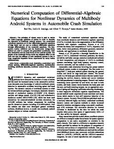
where γ = max{γ− , γ+ } and γ• = sech2 ((2 + α0 )z• + β) for • = + or −. The Fredholm theory of Mallet-Paret [29, 30] is applicable to (3.11) and shows the existence of monotone solutions and a monotone (β, c) curve for c 6= 0. The condition (ii) on page 56 of [30] requires that αj > 0 for all j, while our condition (3.14) implies condition (v), page 56 of [30]. In Figure 3.7 we show the results of some of our numerical experiments. Figure 3.7 is a plot of the function in (3.12) and a plot of a (β, c) curve, the analogue for this problem of an (a, c) curve. beta vs c for Ising with \alpha_0 = 0.1 0.15

1

0.1

0.05

beta

β

0

0

-0.05

α0 = −1 α0 = 0 α0 = 0.1 α0 = 1

−1

−1

-0.1

-0.15

0 z

1

-0.2 -0.15

-0.1

-0.05

0

0.05

0.1

0.15

0.2

c

Fig. 3.7. (i) Plots of 0.5 ln((1 + z)/(1 − z)) − 2 − α0 = 0, for different values of α0 . The roots of (3.12) may thus be determined by intersection with a horizontal line corresponding to values of β. (ii) A (β, c) curve for the Ising model with α0 = 0.1.

14

ABELL, ELMER, HUMPHRIES, AND VAN VLECK

3.5. Frenkel-Kontorova type equations. Consider the Frenkel-Kontorova (FK) type equation [40, 41] (3.15) (3.16)

x ¨j + γ x˙ j = xj−1 − 2xj + xj+1 − d sin xj + F, j = 1, ..., N, xj+N = xj + 2πM.

Here the xj ’s denote the positions of particles in a chain, N is the number of particles, F is an applied force, and M is an arbitrary integer. This equation was first proposed to describe the motion of dislocations in crystals, but is now used to model a number of processes. The equation admits traveling wave solutions, which are referred to as uniform sliding states in the physics literature. Using the traveling wave ansatz xj (t) = ϕ(σj − ct), where σ = 2πM N , equation (3.15),(3.16) becomes (3.17) (3.18)

c2 ϕ(ξ) ¨ − γcϕ(ξ) ˙ = Lσ ϕ(ξ) − d1 sin(ϕ(ξ)) + F, ϕ(ξ + 2π) = ϕ(ξ) + 2πM,

where Lσ ϕ(ξ) = ϕ(ξ − σ) − 2ϕ(ξ) + ϕ(ξ + σ)

and

ξ = σj − ct.

The particular choice of σ is made in order to achieve a simple relationship between the velocity c of the traveling wave and the average particle velocity. The boundary conditions (3.16) imply ¶ µ · ¸¶ µ 2πM 2πM = ϕ σj − c t − = ϕ(σj + 2πM − ct) = ϕ(σj − ct) + 2πM = xj (t) + 2πM. xj t − c c Thus the average particle velocity is −c, the negative of the traveling wave velocity. Because of the discrete translational symmetry in (3.17) it is sufficient to solve (3.17) subject to ϕ(ξ + 2π) = ϕ(ξ) + 2π to obtain solutions to (3.17),(3.18). We choose to solve (3.17) on the interval [−π, π] subject to the conditions (3.19)

ϕ(π) = ϕ(−π) + 2π

and

ϕ(0) = 0

where ϕ(0) = 0 is a phase condition, and specifies a unique phase when ϕ is monotonic. In the case of non-monotonic ϕ (as will arise in this example), this condition no longer guarantees a unique solution to the equations, but in general solutions will be locally unique, a sufficient condition for the numerical convergence. An alternative formulation of this problem is  ¨ − γc[1 + ψ(ξ)] ˙ = Lσ ψ(ξ) − d1 sin(ξ + ψ(ξ)) + F,  c2 ψ(ξ) (3.20) ψ(π) = ψ(−π),  ψ(0) = 0. with

(3.21)

ϕ(ξ) = ξ + ψ(ξ).

The function ψ, referred to as the dynamic hull function, is periodic. We numerically solve both formulations, where we choose F and solve the auxiliary equation c˙ = 0 to find c, as in previous examples. One can also fix c and solve an auxiliary equation F˙ = 0 to find F , which is often easier. In the linear case where d1 = 0 it is simple to verify that ϕ(ξ) = ξ and ψ(ξ) = 0 solve (3.17),(3.19), and (3.20) respectively with F = −γc.

15

COMPUTATION OF MIXED TYPE FUNCTIONAL BVPS Travelling Wave Solutions forγ=0.5

Wave−speed against Forcing for γ=0.5 3 2.5 2

1

2

0

F

φ(ξ)

1.5 −1 c=−8 c=−4 c=−3 c=−2.5 c=−2 c=−1.9 c=−1.875

−2

1

d=0 d=1 d=2 d=3

−3

0.5 −4

−5 0 −4

−3.5

−3

−2.5

−2 c

−1.5

−1

−0.5

0

−3

−2

−1

0 ξ

1

2

3

Fig. 3.8. Solutions of (3.17),(3.19) with γ = 0.5, M = 89, N = 233. (i) Traveling Wave Velocity c against applied Force F for d1 = 1, 2 and 3. (ii) Traveling Wave profiles for d = 2.

Following [40] in Figure 3.8 we present computations for γ = 0.5, M = 89, N = 233 and d 1 = 1, 2 and 3. There is good agreement between the velocity-force characteristics in Figure 3.8(i) and those in Fig 2 of [40], which were computed by a different method. The cusps seen in Figure 3.8(i) are caused by resonances. For −c large, above the first resonance, all the graphs are close to the line F = −γc which corresponds to the linear case d1 = 0. As in the previous examples, propagation failure is numerically resolvable depending on the parameter d1 , with an interval of propagation failure become obvious for d1 large (d1 > 2). In Figure 3.8(ii) we show the evolution of the traveling wave profile as −c is decreased towards the first resonant velocity. For large velocities, motion is essentially linear, but as the traveling wave velocity is decreased becomes less so, and becomes non-monotonic at the first turning point of the graph at −c ≈ 2.5. For d1 = 2 and F ∈ [1.5, 2] it is clear from Figure 3.8(i) that there exist traveling waves with three different wave speeds. We find numerically that only the wave of largest speed is monotonic. In Figure 3.9(i) we show the three traveling waves for F = 1.75. As the wave speed decreases the form of the traveling wave solution becomes progressively more complicated as demonstrated in Figure 3.9(ii). Consider briefly the case M = 1, N = 200, d1 = 2 and γ = 1/20. For this case the first resonant velocity is very small at approximately π/100. Figure 3.10(i) shows the F against c profile to the first resonant velocity. Figure 3.10(ii) shows corresponding traveling wave profiles. For M/N ¿ 1 we obtain step-like traveling wave solutions, much like the behavior seen in the other examples (with the exception that the F (c) curve again fails to be monotonic). 4. Numerical Analysis. In this section we describe the implementation of our methods in the software package COLMTFDE (COLocation for Mixed Type Functional Differential Equations) we are developing, which was used to produce the results presented above, and the numerical analysis issues which arise. COLMTFDE is a collocation boundary value problem solver, and is a member of the COLSYS family [2, 6, 13, 42]. Thus we pay particular attention to the differences between our code and other members of the COLSYS family. The main difference is the ability to handle delayed (and advanced) terms directly. The size of the delays {s σ (x)}nσ=1 and even their number n may be dependent on x. FI in (1.1) can be a fully nonlinear function of uI (x + sσ ) and its derivatives up to and including the m-th derivative (which we made use of in Section 3.4). Also of significance is COLMTFDE’s ability to handle implicitly defined boundary functions, as

16

ABELL, ELMER, HUMPHRIES, AND VAN VLECK Travelling Wave Solutions forγ=0.5 and F=1.75

Travelling Wave Solutions forγ=0.5 3

3

2 2 1 1 0 0 φ(ξ)

φ(ξ)

−1

−2

−1

c≈−3.40 c≈−2.02 c≈−1.78

−3

c=−0.7 c=−0.5 c=−0.3

−2 −4 −3 −5

−6

−4 −3

−2

−1

0 ξ

1

2

3

−3

−2

−1

0 ξ

1

2

3

Fig. 3.9. Solutions of (3.17),(3.19), with γ = 0.5, M = 89, N = 233 and d 1 = 2. (i) Three Traveling Waves for F = 1.75. (ii) Traveling Waves for c = −0.7, c = −0.5, c = −0.3. Wave profile for γ=1/20

Forcing against Wave−speed for γ=1/20 4

0.5

0.45

3

0.4 2 0.35 c=8: ...........

1 0.3 φ(ξ)

F

c=4: −.−.−. 0.25

c=2: −−−−

0

c=1: ____ 0.2

c=0.5: ............

−1

c=0.2: −.−.−.

0.15

c=0.1: −−−−

−2 0.1

c=0.05:____ −3

0.05

0 −8

−4 −7

−6

−5

−4 c

−3

−2

−1

0

−3

−2

−1

0 ξ

1

2

3

Fig. 3.10. Solutions of (3.17),(3.19) with γ = 1/20, M = 1, N = 200 and d 1 = 2. (i) Applied force F against traveling wave velocity c. (ii) Traveling Wave profiles.

described in Section 2.3 as well as explicitly defined boundary functions. COLMTFDE also allows non-separated boundary conditions of the form ∗

(4.1)

m X

J=1

BJ y(ζ(J)) = βJ ,

whereas most of the COLSYS family of BVP solvers require that the boundary conditions for the problem are separated. The introduction of the scalar factors τI (x) multiplying the highest order term on the left-hand side of (1.1) also constitutes a significant generalization from other members of the COLSYS family, further extending the range of problems which may be solved. This is particularly important in problems such as the spatially discrete Nagumo equation where a traveling wave with speed c satisfies (3.4). Two boundary conditions are needed to compute a numerical solution due to the presence of the second-order difference term (ϕ(ξ + 1) − 2ϕ(ξ) + ϕ(ξ − 1)) on the right-hand side of (3.4). However, since there is only a first-order derivative term present, a boundary value problem

COMPUTATION OF MIXED TYPE FUNCTIONAL BVPS

17

solver will only expect and indeed allow one boundary value, which will result in a singular linear system. This difficulty is resolved by introducing a second-order derivative term τ ϕ(ξ) ¨ as in (3.4) and then solving the problem with τ = 0, as in Figure 3.3. Other members of the COLSYS family use local parameter condensation, to eliminate variables which are internal to subintervals of the mesh, thus simplifying the linear system, and reducing storage requirements. They also take advantage of the almost-block-diagonal nature of the resulting linear matrix to solve this system extremely efficiently. However, parameter condensation is not practical for a functional differential equation solver, as the forward and backward delay terms typically fall between collocation points in different mesh intervals, and hence the so-called local variables are no longer truly local. Also, these delay terms will not usually fall on the sub- or super-diagonals of the matrix, and their relative locations will therefore not only depend on the size of the mesh but will require updating with each mesh refinement. The resulting linear matrix will therefore not in general be almost-block-diagonal. COLMTFDE therefore cannot make use of parameter condensation or block diagonal structure. This has significant computational costs, as construction and storage of the full linear matrix, which has size (N (m∗ + kd) + m∗ )2 requires considerably more memory than the condensed matrix, of size N (2m∗ 2 + 3m∗ kd + kd2 ) stored by COLMOD. In addition, since the matrix is no longer sparse almost-block-diagonal we cannot take advantage of efficient solvers for such systems, and use a full forward-backward substitution method. The loss of sparseness cannot be avoided in general, as problems such as the Ising Problem of Section 3.5 will always result in dense matrices. 4.1. Collocation Formulation. We consider a k-stage collocation scheme for (1.1). Let π : T− = x0 < x1 < ... < xN −1 < xN = T+ and hi := xi+1 − xi and h := maxi=0,...,N {hi }. Let {ρi }ki=1 denote k Gaussian collocation points ordered so that 0 6 ρ1 < · · · < ρk 6 1. We seek a collocation solution uπ (x) = (uπ1 , uπ2 , . . . , uπd )T , such that for each I = 1, ..., d, the I-th component uπI (x) is a piecewise polynomial function such that uπi ∈ Pk+mI ,π ∩ C mI −1 (T− , T+ ), where Pk+mI ,π is the space of functions which reduce to polynomials of order k + mI on each of subintervals [xi , xi+1 ] of π, for some k > maxI=1,d mI . The differential equation is satisfied at the kN collocation points xij = xi + hi ρj ,

j = 1, ..., k,

i = 1, ..., N.

mI −1

Note that since Pk+mI ,π ∩ C (T− , T+ ) is of dimension kN + mI , and there are kN collocation conditions associated with the I-th equation, there must be mI side conditions resulting from this equation, and thus m∗ side conditions in total. This exactly matches the number of boundary conditions in (1.1), which uπ is thus required to satisfy. We employ the now standard monomial Runge-Kutta basis representation. Consider a fixed mesh element x ∈ [xi , xi+1 ]. Then, writing u for an arbitrary component uI , and m for mI , I ∈ 1, . . . , d, each polynomial uπ (x) can be expressed in terms of its Taylor series about xi as (4.2)

uπ (x) =

k+m X j=1

k m X X x − xi (x − xi )j−1 (x − xi )j−1 j−1 ψmj ( D uπ (xi ) = yij + hm )zij , i (j − 1)! (j − 1)! hi j=1 j=1

where Dl−1 ψmj (0) Dm ψmj (ρl )

= 0, = δjl ,

1 6 l 6 m, 1 6 j 6 k, 1 6 l 6 k.

18

ABELL, ELMER, HUMPHRIES, AND VAN VLECK

Hence, corresponding to (4.2) yij = Dj−1 uπ (xi ),

1 6 j 6 m,

zij = Dm uπ (xij ),

and

1 6 j 6 k.

and so the collocation solution, uπ , can now be written in terms of yi := (yi1 , . . . , yim )T ,

(4.3)

zi := (zi1 , . . . , zik )T ,

and approximating the solution of (1.1) is reduced to finding these vectors. However even in the linear case the details of the construction of this system are somewhat complicated, and we describe them below. 4.1.1. Linear Systems. The functions FI and GJ in (1.1) are usually non-linear. When they are linear, the system can be written in the form # "m m d t +1 t X X X I (l−1) I (l−1) (mI ) ¯ t (x) + qI (x), ctl (x)D ut (x) + αtl (x)D u γI D uI (x) = t=1

l=1

l=1

with I = 1, . . . , d , x ∈ (T− , T+ ), I I αItl (x) := (αtl (x + s1 (x)), . . . , αtl (x + sn (x)))T ,

and boundary conditions as in (1.1). The process described above leads to a linear system of equations for u π and its first (m − 1) derivatives. We now outline the construction of this system, first for d = 1, and then in the more complicated higher-dimensional case. 4.1.2. One dimensional System. Write the one-dimensional linear delay system as "m+1 # n m X X X (l−1) (l−1) m (4.4) αl (x + sσ )D u(x + sσ ) + q(x), cl (x)D u(x) + τ D u(x) = σ=1

l=1

l=1

and suppose that for some delay sσ , where σ ∈ {1, . . . , n} and some collocation point xir , i ∈ {1, . . . , N }, r ∈ {1, . . . , k}, we have xω 6 xir + sσ < xω+1 , i.e. we identify the mesh interval [xω , xω+1 ] in which the delayed collocation point lies. For convenience, we denote x irσ := xir + sσ , then, from (4.2), we have the following representation for the function uπ and its derivatives at the point xirσ , D(l−1) uπ (xirσ ) =

k m X X xi − x ω (xirσ − xω )j−l m−l+1 yωj + hω D(l−1) ψmj ( rσ )zωj , (j − l)! hω j=1 j=l

Dm u(xirσ ) = hω

k X

Dm ψmj (

j=1

xirσ − xω )zωj . hω

Since uπ must satisfy equation (4.4) at each collocation point xij , applying the collocation equations yields the k equations for yi and zi : −(Vi +

n X

σ=1

Piσ )yi + (Wi −

n X

σ=1

Qσi )zi = qi ,

1 6 i 6 N,

where Vi and Pi are k × m matrices, with entries i Vrj

=

j X cl (xir )(hi ρr )j−l l=1

(j − l)!

,

i Prj

j X αl (xirσ )(xirσ − xω )j−l = , (j − l)! l=1

1 6 r 6 k,

1 6 j 6 m,

19

COMPUTATION OF MIXED TYPE FUNCTIONAL BVPS

and Wi and Qi are k × k matrices, with entries i Wrj

Qirj

= τ δrj −

=

m+1 X

m X

     

cl (xir )hm+1−l D(l−1) ψmj (ρr ), i

l=1

µ

αl (xirσ )hm+1−l D(l−1) ψmj i

l=1

xirσ − xω hω

¶

1 6 r, j 6 k.

  ,   

We let qi := (q(xi1 , . . . , q(xik ))T , and recall that yi and zi were defined in (4.3). From the m global continuity requirements, we obtain the additional relations, Ci yi + Di zi = yi+1 ,

1 6 i 6 N,

where C is a m × m matrix, with entries i = Crj

hij−r , (j − r)!

j>r

and D is of order m × k, with entries i D(r−1) ψmj (1), = hm+1−r Drj i

1 6 r 6 m,

1 6 j 6 k.

We therefore have a linear system for uπ and its first m − 1 derivatives. 4.1.3. Higher Dimensional System. For systems of equations, the situation is more complicated, and the notation becomes rather convoluted. However, it is worth giving in detail, as the construction of the linear matrix for a mixed system is not immediately obvious. Applying the collocation equations for a system with d > 1, yields kd equations for y i and zi , ¯i + −(V

n X

σ=1

¯iσ )yi + (W ¯i − P

n X

σ=1

¯σi )zi = qi , Q

1 6 i 6 N,

¯i is a kd × m∗ matrix, whose entries are themselves matrices, so where V i ¯RJ V = [V i ],

1 6 R 6 k,

1 6 J 6 d,

where V i is a d × mJ matrix with entries i VIj =

j X cIJl (xiR )(hi ρR )j−l , (j − l)!

1 6 I 6 d,

1 6 j 6 mJ .

l=1

¯ i is a kd × kd matrix, with entries again consisting of submatrices, In a similar fashion, W

i WIj = τI δRT δIj

i ¯ RT W = [W i ], 1 6 R, T 6 k, mj X m +1−l (l−1) cIjl (xiR )hi j D ψmj T (ρR ), −

1 6 I, j 6 d.

l=1

¯iσ is an kd × m∗ matrix with d × mJ matrix subentries Also, P iσ ¯RJ P = [P iσ ],

1 6 R 6 k, 1 6 J 6 d,

where

iσ PIj

j I X αJl (xiRσ − xω )j−l = , (j − 1)! l=1

1 6 I 6 d, 1 6 j 6 mJ ,

20

ABELL, ELMER, HUMPHRIES, AND VAN VLECK

¯σi is a kd × kd matrix, with entries again consisting of submatrices, and Q iσ ¯iσ Q RT = [Q ],

1 6 R, T 6 k, µ i ¶ X xRσ − xω mj +1−l (l−1) i I , = D ψ mj T αjl (xrσ )hi hω mj +1

Qiσ Ij

1 6 I, j 6 d.

l=1

¿From the m∗ boundary conditions, we obtain m∗ additional relations, ¯i zi = yi+1 , C¯i yi + D

1 6 i 6 N,

where C¯ is a m∗ × m∗ matrix, with matrix entries i C¯IS = δIS [C i ],

1 6 I, S 6 d,

i Crj =

where

hij−r , (j − r)!

1 6 r 6 mI ,

1 6 j 6 mS .

¯ is of order m∗ × kd, with entries We have that D i ¯IJ = δIS [Di ], D

1 6 I 6 d, 1 6 J 6 k,

with

i I +1−r = hm D(r−1) ψmI J (1), Drs i

1 6 r 6 mI , 1 6 s 6 d.

The resulting linear systems are of the form 

−V1  −C1       −Pi1         ···   B1

−W1 −D1 −Q1i

0 I · ···

··· · · −Vi −Ci

−P11

· −Wi −Di

−Q11

0 I

···

−Q1N

···

n −PN

−Qn N

···

·

·



···

−Pin

−Qn i

· · −VN −CN ·

· −WN −DN

··· ·

1 −PN

···

0 I B m∗

                

y1 z1 . . yi zi . . yN zN yN +1





                =                

q1 0 . . qi 0 . . qN 0 β

                 

4.1.4. Nonlinear Systems. For general nonlinear problems of the form (1.1) our code uses the method of quasilinearisation, which is common to all members of the COLSYS family of codes. The changes made to allow for delay terms to be treated directly are to the construction and storage of the linear system. The method of solving the non-linear problem (1.1) is therefore almost identical to that used for COLMOD [1]. The differences involve the order in which quantities are obtained or constructed due to the backward and forward delay terms. 4.2. Convergence. Assuming sufficient smoothness of the problem coefficients and of the exact solution (except at a finite number of points which form part of the mesh π), much of the standard stability and approximation theory for ODE BVP collocation solutions presented in [3] holds in the presence of delays, with some important changes. A basic convergence result for the solution of delay differential equations of this type by collocation is given in [5], and we reproduce it here. Following [5], in order to keep the notation as simple as possible, the result is given in the case of the first-order equation (4.5)

τ u0 (x) = F (x, u(x), u ¯),

x ∈ (T− , T+ ),

with u ¯I = (u(x + s1 (x)), . . . , u(x + sn (x)))T , and where {sσ (x)}nσ=1 is a finite collection of delays, possibly dependent on x. Generalization to systems of higher order such as (1.1) is straightforward.

COMPUTATION OF MIXED TYPE FUNCTIONAL BVPS

21

The mesh π is defined on the interval [T− , T+ ], such that π : T− = x0 < x1 < ... < xN −1 < xN = T+ , with hi := xi+1 − xi and h := maxi hi . Then, denoting min

x∈[T− ,T+ ]

s1 (x) = T¯− ,

max

x∈[T− ,T+ ]

sn (x) = T¯+ ,

a solution u∗ of (4.5), is in general only a piecewise smooth function for x ∈ [T¯− , T¯+ ], and in fact the solution may be discontinuous at x = T− or x = T+ . To establish convergence assume the right-hand side F of the DDE (4.5) is sufficiently smooth. Then, since the delayed terms {sσ (x)}nσ=1 depend only on x, the locations at which the solution and its derivatives up to order p have potentially non-smooth behavior can be precomputed. Including all these points in the partition π yields u∗ ∈ Cπp [a, b] ∩ C[a, b]. Note that if more smoothness, or in other words a larger p, is required, then the partition π = π(p) becomes more dense in general. The appropriate choice of p for practical computation depends on the BVP and the required accuracy of the numerical solution. The following convergence results for (4.5) are due to Bader [4, 5]. Theorem 4.1. Let u∗ ∈ C p+1 [a, b] for p > 1 be a solution of the problem (4.5) and suppose i) F is sufficiently smooth ii) the linearized problem associated with u∗ is uniquely solvable and has a Green’s function H(x, xi ). Then there exists δ, ε so that a) there is no other solution u ˜ for |D(u∗ − u ˜)| < ε b) for h 6 δ there is a unique collocation solution uπ ∈ Pk+1,π ∩ C[a, b] in this neighborhood of u∗ c) Newton’s method applied to the collocation equations converges quadratically in a neighborhood of uπ for h 6 δ. d) the following error estimates hold for r = 0, 1 |Dr (u − uπ )| 6 κhmin(p,k) e) Furthermore, for the collocation solution of the linearized problem u lin π the following estimates hold min(p,k) |Dr (u − ulin π )| 6 κh

and

2 min(p,k) ). |D r (u − uπ )| = D r (u − ulin π ) + O(h

Proof. See [5] Theorem 2.1: pg.231, and [4]. For ODEs this is usually the departure point in deriving an even higher order of convergence at mesh points, i.e. superconvergence for special sets of collocation points. A crucial basis for all these results is that the Green’s matrix H(x, xi ) has essentially the same smoothness as the solution itself when x 6= xi . This property does not hold for DDEs, see [4] for a simple example. As a consequence, superconvergence can not be shown in general. However, under severe restriction of the class of problems considered and for a special construction of the partition π, superconvergence can be shown to hold. In fact, for superconvergence to occur for DDEs of the form (4.5) the mesh needs to be chosen such that mesh points are mapped into mesh points, and collocation points into collocation points, by the delays. This implies that we can only expect to obtain superconvergence when the sσ ’s are rationally related. This has been further analyzed by Bellen [10] for the special case of initial value problems. However, even if superconvergence is lost, the improvement of order of convergence over approximation techniques is still substantial, since approximation theory uses systems of ODEs to approximate the

22

ABELL, ELMER, HUMPHRIES, AND VAN VLECK

solution of DDEs, and hence attempts to approximate solutions which are only usually piecewise smooth through globally smooth functions (see for example [7]). In contrast with the case of differential equations the error is not necessarily localized when approximating these mixed type delay equations. This impacts the error estimation and hence the mesh selection, and a future improvement will be to address this issue. The error estimation and mesh selection employed are adopted from COLMOD and are described in [42]. Error estimation is based upon the maximum moduli of the left-sided and right-sided approximations to the appropriate derivatives on each subinterval. Mesh selection is based upon so-called semi-equidistribution in which the error over each subinterval is approximately equidistributed. REFERENCES [1] K. A. Abell. Analysis and Computation of the Dynamics of Spatially Discrete Phase Transition Equations. PhD thesis, University of Sussex, 2001. [2] U. Ascher, J. Christiansen, and R. D. Russell. Collocation software for boundary-value ODEs. ACM Trans. Math Soft., 7:209–222, 1981. [3] U. Ascher, R. Mattheij, and R. D. Russell. Numerical Solution of Boundary Value Problems for Ordinary Differential Equations. SIAM, 1995. [4] G. Bader. Numerische Behandlung von Randwertproblemen f¨ ur Funktional-Differentialgleichungen. PhD thesis, University of Heidelberg, 1984. [5] G. Bader. Solving boundary value problems for functional differential equations by collocation. In U.M. Ascher and R.D. Russell, editors, Proceedings in Scientific Computing, Numerical Boundary Value ODEs, volume 5, pages 227–243, 1985. [6] G. Bader and U. Ascher. A new basis implementation for a mixed order boundary value ODE solver. SIAM J. Scient. Stat. Comput., 8:483–500, 1987. [7] H.T. Banks and F. Kappel. Spline approximations for functional differential equations. J. Diff. Eqn., 34:496– 522, 1979. [8] P. Bates and A. Chmaj. On a discrete convolution model for phase transitions. Arch. Rat. Mech. Anal., 150:281–305, 1999. [9] J. Bell. Threshold behaviour and propagation for nonlinear differential-difference systems motivated by modeling myelinated axons. Quart. Appl. Math., 42:1 – 114, 1984. [10] A. Bellen. One step collocation for delay differential equations. J. of Comp. Appl. Math., 10, 1984. [11] W.-J. Beyn. The numerical computation of connecting orbits in dynamical systems. IMA J. Num. Anal., 9:379–405, 1990. [12] J. W. Cahn, J. Mallet-Paret, and E. S. Van Vleck. Travelling wave solutions for systems of ODE’s on a two-dimensional spatial lattice. SIAM J. Appld. Math., 59:455–493, 1999. [13] J.R. Cash, G. Moore, and R.W. Wright. An automatic continuation strategy for the solution of singularly perturbed nonlinear two-point boundary value problems. J. Comp. Phys., 122:266 – 279, 1995. [14] S. N. Chow, J. Mallet-Paret, and W. Shen. Traveling waves in lattice dynamical systems. J. Diff. Eqn., 149:248–291, 1998. [15] F. de Hoog and R. Weiss. An approximation theory for boundary value problems on infinite intervals. Computing, 24:227–239, 1980. [16] C.M. Elliott, A.R. Gardiner, I. Kostin, and Bainian Lu. Mathematical and numerical analysis of a mean-field equation for the Ising model with Glauber dynamics. In P.E. Kloeden and K.J. Palmer, editors, Chaotic Numerics, volume 172 of Contemporary Mathematics, pages 217–242. AMS, 1994. [17] C E Elmer, M Rodrigo, and R M Miura. Constructing Examples: A Technique for Finding Equation/Solution Pairs for Mixed-Type Functional Differential Equations. preprint. [18] C.E. Elmer and E. S. Van Vleck. Analysis and computation of travelling wave solutions of bistable differentialdifference equations. Nonlinearity, 12:771–798, 1999. [19] C.E. Elmer and E. S. Van Vleck. Traveling waves solutions for bistable differential-difference equations with periodic diffusion. SIAM J. Appld. Math., 61:1648–1679, 2001. [20] C.E. Elmer and E. S. Van Vleck. A variant of Newton’s Method for mixed type functional differential equations. J. Dynam. Diff. Eqn., 14:493–517, 2002. [21] K. Engelborghs and E. Doedel. Stability of piecewise polynomial collocation for computing periodic solutions of delay differential equations. Numer. Math., 91:627–648, 2002. [22] K. Engelborghs, T. Luzyanina, K.J. In T Hout, and D. Roose. Collocation methods for the computation of periodic solutions of delay differential equations. SIAM J. Sci. Comp., 22:1593–1609, 2000. [23] B. Fiedler and J. Scheurle. Discretization of Homoclinic Orbits, Rapid Forcing and “Invisible” Chaos. American Mathematical Society, 1996. [24] P. Fife and J. McLeod. The approach of solution of nonlinear diffusion equations to traveling front solutions. Arch. Rat. Mech. Anal., 65:333–361, 1977.

COMPUTATION OF MIXED TYPE FUNCTIONAL BVPS

23

[25] B. Sandstede J. Harterich and A. Scheel. Exponential dichotomies for linear nonautonomous functional differential equations of mixed type. Indiana University Mathematics Journal, 51:1081–1109, 2002. [26] J. P. Keener. Propagation and its failure in coupled systems of discrete excitable cells. SIAM J. Appld. Math., 47:556 – 572, 1987. [27] J. P. Keener. The effects of discrete gap junction coupling on propagation in myocardium. J. Theor. Biol., 148:49 – 82, 1991. [28] M. Lentini and H. B. Keller. Boundary value problems on semi-infinite intervals and their numerical solution. SIAM J. Numer. Anal., 17:577–604, 1980. [29] J. Mallet-Paret. The Fredholm alternative for functional differential equations of mixed type. J. Dyn. Diff. Eqn., 11:1–48, 1999. [30] J. Mallet-Paret. The global structure of traveling waves in spatially discrete dynamical systems. J. Dyn. Diff. Eqn., 11:49–128, 1999. [31] J. Mallet-Paret and S. Verduyn Lunel. Exponential dichotomies and Wiener-Hopf factorizations for mixed-type functional differential equations. J. Diff. Eqn., (to appear), 2003. [32] H.P. McKean. Nagumo’s equation. Advances in Mathematics, 4:209–233, 1970. [33] K. J. Palmer. Exponential dichotomies and transversal homoclinic points. J. Diff. Eqn., 55:225–256, 1984. [34] A. Rustichini. Functional differential equations of mixed type: the linear autonomous case. J. Dyn. Diff. Eqn., 1:121–143, 1989. [35] A. Rustichini. Hopf bifurcations for functional differential equations of mixed type. J. Dyn. Diff. Eqn., 113:145–177, 1994. [36] G. Samaey, K. Engelborghs, and D. Roose. Numerical computation of connecting orbits in delay differential equations. Numer. Alg., 30:335–352, 2002. [37] B. Sandstede. Convergence estimates for the numerical approximation of homoclinic solutions. IMA J. Numer. Anal., 17:437–462, 1997. [38] S. Schecter. Rate of convergence of numerical approximations to homoclinic bifurcation points. IMA J. Numer. Anal., 15:23–60, 1995. [39] L. F. Shampine, R. C. Allen, and S. Pruess. Fundamentals of Numerical Computing. John Wiley, New York, 1997. [40] T. Strunz and F.-J. Elmer. Driven Frenkel-Kontorova model I. uniform sliding states and dynamical domains of different particle densities. Phys. Rev. E, 58:1601–1611, 1998. [41] T. Strunz and F.-J. Elmer. Driven Frenkel-Kontorova model II. chaotic sliding and nonequilibrium melting and freezing. Phys. Rev. E, 58:1612–1620, 1998. [42] R.W. Wright, J.R. Cash, and G. Moore. Mesh selection for stiff two point boundary value problems. Numerical Algorithms, 7:205 – 224, 1994. [43] B. Zinner. Stability of traveling wavefronts for the discrete Nagumo equation. SIAM J. Math. Anal., 22:1016– 1020, 1991. [44] B. Zinner. Existence of traveling wavefront solutions for the discrete Nagumo equation. J. Diff. Eqn., 96:1–27, 1992.