manipulator to automatically select feature points and to derive depth estimates ... and from experiments conducted using the Minnesota. Robotic Visual Tracker ...
Presented at the 1994 IEEE International Conference on Robotics and Automation, May 8-13, 1994, San Diego, CA
Computation of Shape Through Controlled Active Exploration
Christopher E. Smith and Nikolaos P. Papanikolopoulos Artificial Intelligence, Robotics, and Vision Laboratory Department of Computer Science University of Minnesota Minneapolis, MN 55455 Abstract Accurate knowledge of depth continues to be of critical importance in robotic systems. Without accurate depth knowledge, tasks such as inspection, tracking, grasping, and collision-free motion planning prove to be difficult and often unattainable. Traditional visual depth recovery has relied upon techniques that require the solution of the correspondence problem or require known lighting conditions and Lambertian surfaces. In this paper, we present a technique for the derivation of depth from feature points on a target’s surface using the Controlled Active Vision framework. We use a single visual sensor mounted on the end-effector of a robotic manipulator to automatically select feature points and to derive depth estimates for those features using adaptive control techniques. Movements of the manipulator produce displacements that are measured using a Sum-of-Squared Difference (SSD) optical flow. The measured displacements are fed into the controller to alter the path of the manipulator and to refine the depth estimate.
1
Introduction
The computation of the relative and absolute depths of objects’ feature points is essential information for the accurate execution of several robotic manipulation and inspection tasks. Traditional approaches to the problem of depth recovery have assumed that extremely accurate measurements of the camera parameters and the camera system geometry are provided a priori. Such information is not always available or, when it is available, is not always accurate. Inaccuracies are introduced by positioning, path constraints, and environmental changes in the robotic system. Furthermore, camera calibration and the determination of camera parameters can be computationally expensive, time consuming, and error prone. In particular, many depth derivation techniques rely upon stereo vision systems that require careful geometry measurements and the solution of the correspondence problem, making the computational overhead prohibitive for realtime systems. Finally, many structure from motion algorithms use simple accidental motion of the camera that does not guarantee the best possible identifiability of the depth. One solution to these problems can be found under the
Controlled Active Vision framework. Instead of an accidental motion of the eye-in-hand system [8][13][15], we propose a controlled exploratory motion that provides identifiability of the depth parameter. An adaptive controller can be utilized to reduce the influence of such environmental, camera, and manipulator specific inaccuracies to provide accurate and reliable information regarding the depth of an object’s feature points. This information may then be used to guide operations such as tracking, inspection, and manipulation [3][12]. In this paper, we present a technique for the derivation of feature point depth based upon a Sum-of-Squared Differences (SSD) optical flow [1] under an adaptive control framework. The premise behind this technique is that, given an eye-inhand robotic system, features are automatically selected, feature dependent trajectories are produced, and displacements of feature points are measured using the SSD optical flow. These displacements are compared to the predicted displacements that are derived using the current depth estimate. The errors from these comparisons are then used, in conjunction with the previous displacements, to update the depth estimate and to produce the next control input. The control input is derived such that the amount of the error removed in the next iteration will be maximized given environmental and manipulator specific constraints. In this paper, we formulate the equations for optical measurements and the feature point selection scheme. Then, we derive the control and measurement equations used for the adaptive controller and elaborate on the selection of the features’ trajectories. Finally, we discuss results from simulation and from experiments conducted using the Minnesota Robotic Visual Tracker (MRVT).
2
Vision-based measurements and feature selection
2.1
Camera model and optical flow
We assume a pinhole camera model with a world frame, RW, centered on the optical axis and a focal length ƒ. A point P = (XW, YW, ZW)T in RW, projects to a point p in the image plane with coordinates (x, y). We also define two scale factors sx and sy to account for camera sampling and pixel size [12]. Any displacement of the point P can be described by a rota-
tion about an axis through the origin and a translation. If this rotation is small, then it can be described as three independent rotations about the three axes XW, YW, and ZW [2]. We will assume that the camera moves in a static environment with a translational velocity (Tx , Ty , Tz) and a rotational velocity (Rx , Ry , Rz). This results in the following equations for the optical flow (see [12] for a complete derivation): f x u = ------- T z – ------------ T x + ZW sx ZW (2.1)
2
ys y xys y f x s x ----------R x – ---- + ---------- R y + -------R z f f sx sx f y v = ------- T z – ------------ T y + ZW sy ZW
(2.2)
2
xys x xs x f y s y ---- + ---------- Rx – ----------R y – -------R z . f f sy s y
We use a matching based technique known as the Sum-ofSquared Differences (SSD) optical flow [1]. For the point p(k–1) = (x(k–1), y(k–1))T in the image (k–1) where k denotes the kth image in a sequences of images, we want to find the point p(k) = (x(k–1)+u, y(k–1)+v)T. This point p(k) is the new position of the projection of the feature point P in image k. We assume that the intensity values in the neighborhood N of p remain relatively constant over the sequence of k images. We also assume that for a given k, p(k) can be found in an area Ω about p(k–1) and that the velocities are normalized by time T to get the displacements. Thus, for the point p(k–1), the SSD algorithm selects the displacement ∆ x = (u, v)T that minimizes the SSD measure ( p ( k – 1 ), ∆x ) =
∑
m, n ∈ N
[ I k – 1 ( x ( k – 1 ) + m ), y ( k – 1 ) + n ) – I k ( x ( k – 1 ) + m + u, y ( k – 1 ) + n + v ) ]
(2.3) 2
where u,v ∈ Ω, N is the neighborhood of p, m and n are indices for pixels in N, and Ik–1 and Ik are the intensity functions in images (k–1) and (k). The size of the neighborhood N must be carefully selected to ensure proper system performance. Too small an N fails to capture large displacements while too large an N enhances the background, causing inaccurate displacements, and increases the associated computational overhead. In either case, an algorithm based upon the SSD technique may fail due to inaccurate displacements. An algorithm based upon the SSD technique may also fail due to repeated patterns in the intensity function of the image or due to large areas of uniform intensity in the image. Both cases can provide multiple matches within a feature point’s neighborhood, resulting in spurious displacement measures. In order to avoid this problem, the system automatically evaluates and selects feature points.
2.2
Feature point selection
Feature points selection is based upon a confidence mea-
sure derived using the SSD measure and an auto-correlation technique. The neighborhood N , centered upon a prospective feature point in image Ik , is used to collect SSD measures at offsets belonging to the area Ω , also in I k [1][12]. This produces a surface of SSD measures over the area Ω . Several possible confidence measures can be applied to the surface to measure the suitability of the potential feature point. The selection of a confidence measure is critical since many such measures lack the robustness required by changes in illumination, intensity, etc. We utilize a two-dimensional displacement parabolic fit that attempts to fit a parabola (e(∆xr) = a∆xr2+b∆xr+c) to a cross-section of the SSD surface in several predefined directions, producing a measure of the goodness of the fit. Papanikolopoulos [12] selected a feature point if the minimum directional measure was sufficiently high. For instance, a corner point produces an SSD surface with very good parabolic fits in all directions. Such a point is selected since the minimal directional measure will be high. A point belonging to an edge would not be selected since the fit in the direction along the edge would be poor due to multiple matches for the prospective feature point. We extend this approach in response to the aperture problem [7]. Briefly stated, the aperture problem refers to the motion of points that lie on a feature such as an edge. Any sufficiently small local measure of motion can only retrieve the component of motion orthogonal to the edge. Any component of motion due to movement other than that perpendicular to the edge is unrecoverable due to multiple matches for any given feature point. The improved confidence measure for feature points permits the selection of a feature if it has a sufficiently high correlation with the parabola in a particular direction. For instance, a feature point corresponding to an edge will be selected due to the high measure in the direction perpendicular to the edge. This directional information is then used during the depth recovery process to constrain the motion of the manipulator. A corner feature would therefore allow manipulator motion in any direction while an edge feature would constrain motion to the direction perpendicular to the edge. This ensures that the only component of resulting motion is precisely the component that can be recovered under consideration of the aperture problem. This ideal motion is not always achievable; therefore, matches that lie closer to the ideal manipulator motion will be preferred, if multiple matches are detected.
3
Depth recovery modeling
Several robotic servoing problems require accurate information regarding the depth of the object of interest. When this depth is not provided a priori, it must be recovered from observations of the environment via sensing. Traditional depth recovery techniques in a robotic system may suffer from various problems, including computational overhead, expensive calibration, frequent recalibration, obstruction, and solution of the correspondence problem. We present an alternative algorithm for depth recovery using the Controlled
Active Vision framework. Consider a target object at an unknown depth with a feature point, P, located on the surface of the object. The point T P = ( XW, Y W, Z W ) projects onto a camera’s image plane at point p with coordinates (x, y). By moving the visual sensor, a sequence of images and the respective projections of P can be produced. By observing the changes of P’s projections, p(k) and p(k–1), in two successive images (k) and (k– 1), respectively, an estimate of the depth of P is derived. Over multiple images, this estimate can be refined using adaptive techniques. Previous work in depth recovery using active vision relied upon random camera displacements to provide displacement changes in the p(k)’s [4][8][9][13][15][16]. In our approach, we select features automatically, produce feature trajectories (a different trajectory for every feature), and predict future displacements using the depth estimate. The errors in these predicted displacements, in conjunction with the estimated depth, are included as inputs in the control loop of the system. Thus, the next calculated movement of the system produces a camera movement that will eliminate the largest possible portion of the observed error while adhering to various environmental and manipulator specific constraints. This purposeful movement of the visual sensor provides more accurate depth estimates and a faster convergence of the depth measures over a sequence of estimates.
3.1
Formulation of depth recovery
We begin by modeling the depth recovery problem. We will use the SSD optical flow to measure displacements of feature points in the image plane. For a single feature point, p, we assume that the optical flow at time instant kT is (u(kT), v(kT)), where T is the time between two successive frames. It can be shown that at time instant kT, the optical flow is given by: u ( kT ) = u o ( kT ) + u c ( kT )
(3.1)
v ( kT ) = v o ( kT ) + v c ( kT ).
(3.2)
Since we are recovering the depth of feature points on a static object, the components of optical flow due to the movement of the object (uo(kT) and vo(kT)) are zero. Also, equations (3.1) and (3.2) do not account for the computational delays involved with the calculation of the optical flow. By taking these delays into account, and by eliminating the flow components due to object motion, these equations become u ( kT ) = u c ( ( k – d + 1 )T )
(3.3)
v ( kT ) = v c ( ( k – d + 1 )T )
(3.4)
where d is the computational delay factor (d ∈ {1,2,...}). In order to simplify the notation, the index k will be used instead of kT. By utilizing the relations x( k + 1 ) – x( k) y( k + 1 ) – y( k ) u ( k ) = ------------------------------------, v ( k ) = -----------------------------------T T
the equations can be rewritten as: x ( k + 1 ) = x ( k ) + Tu c ( k – d + 1 )
(3.5)
y ( k + 1 ) = y ( k ) + Tvc ( k – d + 1 ).
(3.6)
Furthermore, we can include the inaccuracies of the model (e.g., neglected accelerations, inaccurate robot control) as white noise. The equations (3.5) and (3.6) become x ( k + 1 ) = x ( k ) + Tu c ( k – d + 1 ) + ξ x ( k )
(3.7)
y ( k + 1 ) = y ( k ) + Tv c ( k – d + 1 ) + ξ y ( k )
(3.8)
where ξx ( k ) and ξ y ( k ) are zero mean, mutually uncorrelated, 2 2 stationary random variables with variances σ x and σ y respectively. The above equations may be written in state-space form as p ( k + 1 ) = A ( k )p ( k ) + B ( k – d + 1 )u c ( k – d + 1 ) + H ( k )v ( k )
(3.9) 2
A ( k ) = H ( k ) = I 2 , p ( k ) and v ( k ) ∈ R , and 6 6 u c ( k – d + 1 ) ∈ R . The matrix B ( k ) ∈ R is given by:
where
T
–f ------------Z (k)s W x 0
2 x( k)y(k) s x (k)s y(k) s x(k) x ----------- ------------------y – -s-f + ----------------------y f f sx x Z (k) W . 2 y (k) s –x ( k ) y ( k ) sx x (k ) s y(k) y x f – f -------------- ----------- -s- + --------------------------------– ---------f f s y Z (k )s Z (k) y W y W 0
The vector p ( k ) = ( x ( k ), y ( k ) )
(3.10)
T
is the state vector, T is the control input vector (only movement in the x-y plane of the T end-effector frame is used), and v ( k )= ( ξ x ( k ), ξ y ( k ) ) is the white noise vector. 6 The term, B ( k – d + 1 )u c ( k – d + 1 ) ∈ R can be simplified to u c ( k – d + 1 ) = ( Tx ( k – d + 1 ), T y ( k – d + 1 ), 0, 0, 0, 0 )
B ( k – d + 1 )u c ( k – d + 1 ) = T
–f ------------ T ( k – d + 1 ) ZW sx x
(3.11)
–f ------------ T ( k – d + 1 ) ZW sy y
since ZW does not vary over time and only the T x ( k – d + 1 ) and T y ( k – d + 1 ) control inputs are used. By substitution into equation (3.9) and simplification, we derive the following: x( k
+ 1) = y( k + 1)
x( k) y( k)
+T
–f ----------- T x ( k – d + 1 ) ZW s x –f ----------- T y ( k – d + 1 ) ZW s y
+
ξx ( k ) ξy ( k )
. (3.12)
The previous equation is used under the assumption that the optical flow induced by the motion of the camera does not change significantly in the time interval T. Additionally, the interval T should be as small as possible so that the relations that provide T x ( k – d – 1 ) and T y ( k – d + 1 ) are as accurate as possible. The parameter T has as its lower bound 16 msec (the sampling rate of standard video equipment). If the upper bound on T can be reduced such that it is lower than the sampling rate of the manipulator controller (in our case, 28 msec for the PUMA 560), then the system will no longer be constrained by the speed of the vision hardware. The objective is to design a specific trajectory (a set of T desired p∗ ( k ) = ( x∗ ( k ), y∗ ( k ) ) for successive k’s) for every individual feature in order to identify the depth parame-
ter ZW. Thus, we have to design a control law that forces the eye-in-hand system to track the desired trajectory for every feature. Based on the information from the automatic feature selection procedure, we select a trajectory for the feature. For example, the ideal trajectory for a corner feature is depicted in Figure 1. If the feature belongs to a vertical edge, then y∗( k ) is held constant at y∗init . Then, the control objective function is selected to be
tation is completed, it is trivial to compute the parameter 1 ⁄ Z W that is needed for the construction of the depth maps. It is assumed that the matrix N ( k ) is constant ( N ( k ) = N ). We use the estimation scheme described in [8][10] (for one feature point) p
p
T
F o ( k + d ) = E { ( p m ( k + d ) – p∗ ( k + d ) ) Q ( p m ( k + d ) – p∗ ( k + d ) ) + u c ( k )Ld u c ( k )} } T
i =d–1
Bˆ ( k – i )u c ( k – i ) }
(3.14)
i=1
where Bˆ ( k ) is the estimated value of the matrix B ( k ) . The matrix Bˆ ( k ) depends on the estimated value of the depth Zˆ W . The estimation of the depth parameter is performed by using the procedure described in [12]. In order to use this procedure, we must rewrite equation (3.12) as follows (for one feature point): ∆p m ( k ) = ζW u cnew ( k – d ) + n ( k )
where
(3.15)
∆p m ( k ) = p m ( k ) – p m ( k – 1 ) ζW = f ⁄ ( sx ZW ) n ( k ) ∼ N ( 0 , N( k ) ) – Tx ( k ) . u cnew ( k ) = T – s x ------ Ty( k ) s y
The objective of the estimation scheme is to estimate the parameter ζ W for each individual feature. When this compu-
x* (k) x*max x*init
y* (k)
k1
k2
kF
k1
k2
kF
(3.17)
–1 p T –1 pr ( k ) = ( pr ( k ) ) + u cnew ( k – d )N
u cnew ( k – d ) } T
k
y*max y*init
k Figure 1: Desired trajectories of the features
u
T
u
–1
p T ζˆ W ( k ) = ζˆ W ( k ) + g ( k ) { ∆p m ( k ) – p
(3.18)
–1
g ( k ) = pr ( k ) u cnew ( k – d )N
–1 T ˆ
∑
pr ( k ) = pr ( k – 1 ) + s ( k – 1 ) u
u c ( k ) = – [ B ( k )QBˆ ( k ) + L d ] B ( k )Q { ( p m ( k ) – p∗ ( k + d ) ) +
(3.16)
u
(3.13)
where E { Y } denotes the expected value of the random variable Y, p m ( k ) is the measured state vector, and Q, Ld are control weighting matrices. Based on the equation (3.12) and the minimization of the control objective function F o ( k + d ) (with respect to the vector u c ( k ) , we can derive the following control law ˆT
u ζˆ W ( k ) = ζˆ W ( k – 1 )
(3.19)
(3.20)
ζˆ W ( k )u cnew ( k – d ) }
where the superscript p denotes the predicted value of a variable, the superscript u denotes the updated value of a variable, and s (k) is a covariance scalar. The initial conditions are p described in [12]. The term pr ( 0 ) can be viewed as a measure of the confidence that we have in the initial estimate p ζW ( 0 ) . The next section describes several simulation and experimental results using this scheme.
4
Simulation and experiments
4.1
Simulation results
The model was initially verified in simulation experiments. Simulations were performed on a Silicon Graphics Indigo. The camera and manipulator were modeled, as was the target and the environment. The target was displayed in depth and was projected using a pinhole camera model. It appeared in front of a regular textured background that was placed at optical infinity. The camera was modeled using the perspective transformation of the Indigo’s geometry engine to correspond to a 7.5 mm focal length lens and an image plane that was sized to correspond to a 1/2″ CCD camera array. The image plane was placed in front of the nodal point of the optical system due to the modeling specifically used by the Indigo. The manipulator was modeled using second-order partial differential equations that transform the ideal control vector into a realized control vector based upon the current motion vector of the manipulator. The initial simulation runs were conducted with a sodacan sized cylinder placed 45 cm in depth. The controller began the depth extraction process with an initial depth parameter estimate of 1 meter. The recovery process consisted of a sequence of motions, each producing an image. Once completed, the recovered depth of each feature point was compared to the actual depth to produce a measure of the accuracy of the process. For virtually all feature points, the variation of the recovered versus the computed was subpixel in nature. In fact, the majority of the sub-pixel errors were
CCD Camera Unimation Controller
Arm/Controller Cable
Sun 4/330 B I T 3
Figure 2: Single target surface less than one half of the error calculated for a given displacement error of one pixel. It should be noted that sub-pixel fitting and multi-grid methods were not employed in this process due to their computational overhead. The reconstructed surface is shown in Figure 2. A second set of simulation runs were conducted using two soda-can sized cylinders. The first cylinder was rendered at 45 cm in depth. The second was rendered at 70 cm in depth. Again, a regular textured background was placed at optical infinity. The initial depth parameter estimate was set to 1 meter. The results of the process were again highly accurate, achieving sub-pixel accuracy for virtually all the selected feature points. The result of the surface reconstruction is shown in Figure 3. The reconstruction retains the perspective effect upon the apparent relative size of the targets; thus, the target at greater depth appears smaller.
4.2
Hardware results
Once we determined that the performance of the simulation was satisfactory, the algorithm was implemented on the Minnesota Robotic Visual Tracker (MRVT) (see Figure 4). The system consists of a PUMA 560 manipulator controlled via the Unimation Controller’s alter line. The alter line requires path control updates once every 28 msec. Those updates are provided by an Ironics 68030 VME processor that shares its bus with a Sun Sparc 330 and a Datacube vision system via BIT-3 bus extenders. A Panasonic miniature camera is mounted parallel to the end-effector of the PUMA and provides its output to the Datacube for processing. The Datacube system consists of a MVME-147 processor, a MaxVideo 20 video processor, and a Max860 vector processor. The vision sub-system performs the optical flow, calculates the input control vector according to the control law, and sup-
Figure 3: Dual target surface
B I T 3
VME I V B 3 I 2 T 3 3 0
Datacube M a M B M a 1 I x x 4 T 2 8 7 3 0 6 0
Figure 4: MRVT system architecture plies the input vector to the Ironics processor for transmission to the Unimate controller. The initial experimental runs were conducted with a sodacan wrapped in a matte, checkerboard covering and was placed in depth such that the leading edge of the curved surface was 53 cm from the nodal point of the camera (see Figure 5). Similar to the simulation experiments, the initial depth estimate was set to 1 meter of depth. The modelling for the visual process was precisely the same as in the simulation runs; however, the camera scaling factors and the controller gains were changed to meet the specifications of the miniature camera and the PUMA manipulator. Again, the resulting data for the feature points was not subjected to sub-pixel fitting nor multi-grid methods. It should be noted that, similar to the simulation, the error in the recovered depth of the majority of feature points was subpixel in nature. The reconstructed surface of the single soda can is shown in Figure 6. A second set of experiments was also conducted in the same fashion as the simulations, using two soda cans as targets. The leading edges of the cans were placed at 53 cm and 41 cm in depth (see Figure 7). Again, the majority of the errors in the calculated depths were sub-pixel. For these runs, the initial depth estimate was an underestimate of 25 cm, in contrast to the previous simulations and experiments that used overestimates. The reconstructed surfaces of the dual can experiment are shown in Figure 8. Further experimental results using real surfaces (rather
Figure 5: Single can target
Figure 6: Single can surface than the matte checkerboards) can be found in [14].
5
Conclusion
This paper presents a novel technique for computing depth maps through controlled active exploration with a camera. Unlike similar approaches [6][8][9][13][15], we propose a scheme that is based on automatic selection of features and design of specific trajectories on the image plane for each individual feature. This approach helps us design trajectories that provide maximum identifiability of the depth parameter. During the execution of the specific trajectory, the depth parameter is computed with the help of a simple estimation scheme that takes into consideration the previous movements of the camera and the computational delays. The approach has been tested with simulations and experiments, and several experimental results have been presented. Issues for future research include the automatic selection of the window size (an issue discussed in [11]) in order to select a window that has some texture variations, the computational improvement of the approach, and the implicit incorporation of the robot dynamics.
6
Acknowledgments
This work has been supported by the Department of Energy (Sandia National Laboratories) through Contract #AC-3752D, the Center for Advanced Manufacturing, Design, and Control (CAMDAC) of the University of Minnesota, the Center for Transportation Studies through Contract #USDOT/DTRS93-G-0017-01, the 3M Corporation, the
Figure 8: Dual can surface Graduate School of the University of Minnesota, and the Department of Computer Science at the University of Minnesota.
7
References
[1]
P. Anandan, “A computational framework and an algorithm for the measurement of visual motion,” International Journal of Computer Vision, 2(3):283-310, 1988. J.J. Craig, Introduction to robotics: mechanics and control, Addison-Wesley, Reading, MA, 1985. J.T. Feddema and C.S.G. Lee, “Adaptive image feature prediction and control for visual tracking with a hand-eye coordinated camera,” IEEE Transactions on Systems, Man, and Cybernetics, 20(5):1172-1183, 1990. C.P. Jerian and R. Jain, “Structure from motion—a critical analysis of methods,” IEEE Transactions on Systems, Man, and Cybernetics, 21(3):572-588, 1991. J. Heel, “Dynamic motion vision,” Robotic and Autonomous Systems, 6(3):297-314, 1990. K.N. Kutulakos and C.R. Dyer, “Recovering shape by purposive viewpoint adjustment,” Proceedings of the IEEE Conference on Computer Vision and Pattern Recognition, 16-22, 1992. D. Marr, Vision, W.H. Freeman and Company, San Francisco, CA, 1982. L. Matthies, T. Kanade, and R. Szeliski, “Kalman filterbased algorithms for estimating depth from image sequences,” International Journal of Computer Vision, 3(3):209-238, 1989. L. Matthies, “Passive stereo range imaging for semi-autonomous land navigation,” Journal of Robotic Systems, 9(6):787-816, 1992. P.S. Maybeck, Stochastic models, estimation, and control, Vol. 1, Academic Press, Orlando, FL, 1979. M. Okutomi and T. Kanade, “A locally adaptive window for signal matching,” International Journal of Computer Vision, 7(2):143-162, 1992. N. Papanikolopoulos, “Controlled active vision,” Ph.D. Thesis, Department of Electrical and Computer Engineering, Carnegie Mellon University, 1992. C. Shekhar and R. Chellappa, “Passive ranging using a moving camera,” Journal of Robotic Systems, 9(6):729-752, 1992. C. Smith, S. Brandt, and N. Papanikolopoulos, “Controlled Active Exploration of Uncalibrated Environments,” To appear, Proceedings of the IEEE Conference on Computer Vision and Pattern Recognition, 1994. C. Tomasi and T. Kanade, “Shape and motion from image streams under orthography: a factorization method,” International Journal of Computer Vision, 9(2):137-154, 1992. D. Weinshall, “Direct computation of qualitative 3-D shape and motion invariants,” IEEE Trans. on Pattern Analysis and Machine Intelligence, 13(12):1236-1240, 1991.
[2] [3]
[4] [5] [6]
[7] [8]
[9] [10] [11] [12] [13] [14]
[15] [16]
Figure 7: Two can target