Computational Experience with a Software Framework for Parallel Integer Programming Y. Xu∗
T. K. Ralphs†
L. Lad´anyi‡
M. J. Saltzman§
September 25, 2007
Abstract In this paper, we discuss the challenges that arise in parallelizing algorithms for solving mixed integer linear programs and introduce a software framework that aims to address these challenges. The framework was designed specifically with support for implementation of relaxationbased branch-and-bound algorithms in mind. Achieving efficiency for such algorithms is particularly challenging and involves a careful analysis of the tradeoffs inherent in the mechanisms for sharing the large amounts of information that can be generated. We present computational results that illustrate the degree to which various sources of parallel overhead affect scalability and demonstrate that properties of the problem class itself can have a substantial effect on the efficiency of a particular methodology.
1
Introduction
In this paper, we discuss a framework for parallelization of algorithms based on branch and bound for solving general mixed integer linear programs (MILPs). We focus particularly on branch and cut, which is currently the most effective and commonly used approach for solving difficult MILPs. Despite this, however, many MILPs arising in practice remain difficult to solve by branch and cut. The difficulty stems mainly from limitations in memory and processing power, so a natural approach to overcoming this difficulty is to consider the use of so-called “high-throughput” computing platforms, which can deliver a pooled supply of computing power and memory that is virtually limitless. Branch and bound employs a divide-and-conquer strategy that partitions the original solution space into a number of smaller subsets and then analyzes the resulting smaller subproblems in a recursive fashion. Such an approach appears easy to parallelize, but this appearance is deceiving. Although it is easy in principle to divide the original solution space into subsets, it is difficult to do this in a way such that the amount of effort required to solve each of the resulting smaller subproblems ∗
Analytical Solutions, SAS Institute, Cary, NC 27513,
[email protected] Department of Industrial and Systems Engineering, Lehigh University, Bethlehem, PA 18015,
[email protected], http://www.lehigh.edu/~tkr2, funding from NSF grant DMI-0522796 ‡ Department of Mathematical Sciences, IBM T. J. Watson Research Center, Yorktown Heights, NY 10598,
[email protected] § Department of Mathematical Sciences, Clemson University, Clemson, SC 29634
[email protected], http://www.math.clemson.edu/~mjs †
is approximately equal. If the work is not divided equally, then some processors will become idle long before the solution process has been completed, resulting in reduced effectiveness. Even if this challenge is overcome, it still might be the case that the total amount of work involved in solving the subproblems far exceeds the amount of work required to solve the original problem on a single processor. In the remainder of the paper, we describe a framework for meeting the challenges that arise in implementing sophisticated parallel versions of branch and bound, such as branch and cut. The work builds and attempts to improve upon previous efforts, most notably the frameworks SYMPHONY and COIN/BCP, both straightforward implementations employing centralized mechanisms for control of task distribution and information sharing [40, 41]. The paper is organized as follows. In Section 2, we introduce necessary terms and definitions. In Section 3, we describe the implementation details of the COIN-OR High Performance Parallel Search Framework (CHiPPS), a C++ class library developed based on the concepts of knowledge discovery and sharing. In Section 4, we analyze computational results obtained using the framework to solve MILP instances with a wide range of scalability properties. Finally, in Section 5, we conclude and summarize the material presented in the rest of the paper.
2
Definitions and Terms
Mixed Integer Linear Programs. We review here just the basic definitions. For a complete treatment of mixed integer linear programming and associated algorithms, see [37]. A mixed integer linear program is the problem of optimizing a linear objective function over a polyhedral feasible region with the additional constraint that some of the variables are required to take on integer values. More formally, a MILP is a problem of the form zIP =
min
x∈P∩(Zp ×Rn−p )
c⊤ x,
(1)
where P = {x ∈ Rn | Ax = b, x ≥ 0} is a polyhedron defined by constraint matrix A ∈ Qm×n and right-hand side vector b ∈ Qm , and c ∈ Rn is the objective function vector. The variables indexed 1 through p are the integer variables and the variables indexed p + 1 through n are then the continuous variables. The case in which all variables are continuous (p = 0) is called a linear program (LP). Associated with each MILP is an LP, called the LP relaxation, with feasible region P, obtained by relaxing the integrality restrictions. Tree Search Problems. Tree search problems are any of a general class in which the nodes of a directed, acyclic graph must be systematically searched in order to locate one or more goal nodes. The graph must have a unique root node with no incoming arcs, which is the first node to be examined. In such an algorithm, the search order uniquely determines a rooted tree called the search tree in which there is a unique path to each node from the root. In describing tree search problems, it is convenient to distinguish between feasibility problems and optimization problems. Optimization problems are those in which there is a cost associated with the path from the root node to each goal node and the object is to find a goal node that has minimum path cost. For example, the path cost in branch and cut would be interpreted as the difference in bound between the root node and a given search tree node. To specify a tree search algorithm, we must have (1) a processing method that determines whether a node is a goal node and whether it has any successors, 2
(2) a branching method that specifies how to generate the descriptions of a node’s successors, if it has any, and (3) a search strategy that specifies the processing order of the candidate nodes. Tree search algorithms are again easy to parallelize in principle. However, factors such as those described above can confound efforts to achieve efficient parallelization. In [39] and [42], we examined the issues surrounding parallelization of general tree search algorithms and presented high-level procedures for implementing such algorithms. High-Throughput Computing. High-throughput computing is a computing paradigm in which the goal is to effectively harness the very large amounts of (distributed) computing power typically available in modern computing environments. The challenge is to bring multiple, distributed commodity computing resources together to bear on a single problem of interest in an effective manner. The ability to do this depends on properties of the computing environment itself and the tools provided to exploit that environment. Historically, many specialized architectures have been designed and many highly tuned algorithms developed, but recent trends have been toward the use of commodity hardware to construct so-called Beowulf clusters [9]. In this paper, a simplified parallel architecture similar to that of a typical Beowulf cluster is assumed. The important assumptions of such an architecture are (1) that it is homogeneous (all nodes are identical), (2) that it has an “all-to-all” communications network in which any two nodes can communicate directly, (3) that it has no shared access memory, and (4) that it has no global clock by which to synchronize calculations. On such an architecture, all communication and synchronization activities must take place through the explicit passing of “messages” between processors using a message-passing protocol. The two most common message-passing protocols are PVM [15] and MPI [19]. In our simplified model, the two main resources required for computation are memory and processing power, which can be increased only by adding processing nodes to the cluster. A processing node consists of both a CPU (typically called a processor) and associated memory, but we assume that each processing node has sufficient memory for required calculations and will refer to processing nodes simply as processors. Scalability. The primary goal of high-throughput computing is to take advantage of increased processing power to solve problems faster. The scalability of a parallel algorithm (in combination with a specific parallel architecture) is the degree to which it is capable of effectively utilizing increased computing resources (usually processors). The traditional way to measure scalability is to compare the speed with which we can execute a particular algorithm on p processors to that with which we could solve it on a single processor. The sequential running time (S) is used as the basis for comparison and is usually taken to be the wall clock running time of a sequential implementation of the algorithm. The parallel running time (Tp ) is the wall clock running time of the parallel algorithm running on p processors. The speedup (Sp ) is the ratio S/Tp . Finally, the efficiency (Ep ) is the ratio Sp /p of speedup to number of processors. Note that all these quantities depend on p. The aim is then to maintain an efficiency as close to one as possible as the number of processors is increased. The loss of efficiency that occurs as the number of processors is increased comes both from extra work that must be performed in the parallel algorithm and time that processors spend idle when they might be doing useful work. More specifically, the main types of overhead we consider are: • Idle time (ramp-up/ramp-down): Time spent by processors waiting for their first task to be allocated or waiting for termination at the end of the algorithm. 3
• Idle time (synchronization/handshaking): Time spent waiting for information requested from another processor or waiting for another processor to complete a task. • Communication overhead : Processing time associated with sending and receiving information, including time spent inserting information into the send buffer and reading it from the receive buffer at the other end. • Performance of redundant work : Processing time spent performing work (other than communication overhead) that would not have been performed in the sequential algorithm. It is important to point out that every algorithm has a certain portion that is inherently sequential. Amdahl called this portion of the running time the sequential fraction [3]. Because of this fact, the efficiency with which problems of similar size and difficulty can be solved drops as the number of processors increases. This is because the sequential fraction comes to represent an increasingly large percentage of the wallclock running time. If the number of processors is kept constant, then efficiency generally increases as problem size increases [18, 20, 26]. This led Kumar and Rao to suggest a measure of scalability called the iso-efficiency function [27], which measures the rate at which the problem size has to be increased with respect to the number of processors in order to maintain a fixed efficiency. Such a function provides perhaps the most accurate overall picture of scalability, but computing it is problematic for a number of reasons that will be made clear later. Knowledge. We refer to potentially useful information generated during the execution of the algorithm as knowledge. Trienekens and de Bruin introduced the notion that the efficiency of a parallel algorithm is inherently dependent on the strategy by which this knowledge is stored and shared among the processors [47]. From this viewpoint, a parallel algorithm can be thought of roughly as a mechanism for coordination of a set of autonomous agents that are either knowledge generators (KGs) (responsible for producing new knowledge), knowledge pools (KPs) (responsible for storing previously generated knowledge), or both. Specifying such a coordination mechanism consists of specifying what knowledge is to be generated, how it is to be generated, and what is to be done with it after it is generated (stored, shared, discarded, or used for subsequent local computations). Tasks. Just as KPs can be divided by the type of knowledge they store, KGs may be divided either by the type of knowledge they generate or the method by which they generate it. In other words, processors may be assigned to perform only a particular task or set of tasks. If a single processor is assigned to perform multiple tasks simultaneously, a prioritization and time-sharing mechanism must be implemented to manage the computational efforts of the processor. The granularity of an algorithm is the size of the smallest task that can be assigned to a processor. Choosing the proper granularity can be important to efficiency. Too fine a granularity can lead to excessive communication overhead, while too coarse a granularity can lead to excessive idle time and the performance of redundant work. We have assumed an asynchronous architecture, in which each processor is responsible for autonomously orchestrating local algorithm execution by prioritizing local computational tasks, managing locally generated knowledge, and communicating with other processors. Because each processor is autonomous, care must be taken to design the entire system so that deadlocks, in which a set of processors are all mutually waiting on one another for information, do not occur.
4
2.1
Previous Work
The branch and bound algorithm was first suggested by Land and Doig in 1960 [28]. In 1970, Mitten abstracted branch and bound into the theoretical framework we are familiar with today [35]. However, it was another two decades before sophisticated software packages for solving MILPs began to be developed. Most of the software packages currently available implement some version of the branch and cut algorithm. Available noncommercial generic MILP solvers include bonsaiG [21], CBC [14], GLPK [24], lp solve [32], MINTO [36], and SYMPHONY [41]. Commercial MIP solvers include ILOG’s CPLEX and Dash’s XPRESS. Generic frameworks that allow the user to take advantage of special structure by implementing specialized functionality, such as problem-specific cut generation, include SYMPHONY, COIN/BCP [40], ABACUS [23], and CBC. CONCORDE [4, 5], a package for solving the traveling salesman problem, also deserves mention as the most sophisticated special-purpose code developed to date. Numerous software packages implementing parallel branch and bound and parallel branch and cut have also been developed. The previously mentioned SYMPHONY, COIN/BCP, and CONCORDE all have parallel execution modes and can be run on networks of workstations. Other related software includes frameworks for implementing parallel branch and bound such as PUBB [44], BoB [7], PPBB-Lib [48], PEBBL [12] (formerly PICO), and OOBB [17]. PARINO [31] and FATCOP [10] are parallel generic MILP solvers.
3
The COIN-OR High Performance Parallel Search Framework
The COIN-OR High Performance Parallel Search (CHiPPS) Framework is a C++ class library hierarchy for implementing customized versions of parallel tree search. The central core of CHiPPS is a library of base classes known as the Abstract Library for Parallel Search (ALPS) (see Section 3.1). Because of its general approach, ALPS supports the implementation of a wide variety of algorithms and applications by creating application-specific derived classes implementing the algorithmic components required to specify a tree search. Prototypes of two specialized solvers built directly with ALPS, one for solving the well-known knapsack problem and one for solving generic MILPs, have been developed and previously reported on [49]. We discuss here the details of two additional C++ class libraries derived from ALPS that add to CHiPPS the functionality needed for relaxation-based branch and bound for mathematical programming. The Branch, Constrain, and Price Software (BiCePS) library adds the data handling and bookkeeping capabilities needed for relaxation-based solution methods for mathematical programming problems (see Section 3.2). The BiCePS Linear Integer Solver (BLIS) library is a concretization of BiCePS for solving mixed integer linear programs (see Section 3.3).
3.1 3.1.1
ALPS Knowledge Management
Knowledge Objects. ALPS takes an almost completely decentralized approach to knowledge management. The fundamental concepts of knowledge discovery and sharing are the basis for the class structure of ALPS, shown in Figure 1 (along with the class structure for BiCePS and BLIS). In this figure, the boxes represent classes, an arrow-tipped line connecting classes represents 5
Figure 1: Library Hierarchy of CHiPPS
6
an inheritance relationship, and a diamond-tipped line connecting classes indicates an inclusion relationship. A central notion in ALPS is that all information generated during execution of the search is treated as knowledge and is represented by objects of C++ classes derived from the common base class AlpsKnowledge. This class is the virtual base class for any type of information that must be shared or stored. AlpsEncoded is an associated class that contains the encoded or packed form of an AlpsKnowledge object. The packed form consists of a bit array containing the data needed to construct the object. This representation takes less memory than the object itself and is appropriate both for storage and transmission of the object. The packed form is also independent of type, which allows ALPS to deal effectively with user-defined or application-specific knowledge types. To avoid the assignment of global indices, ALPS uses hashing of the packed form as an effective and efficient way to identify duplicate objects. ALPS has the following four native knowledge types, which are represented using classes derived from AlpsKnowledge. • AlpsModel: This class contains the data describing the original problem. This data is shared globally during initialization and maintained locally at each processor during the course of the algorithm. • AlpsSolution: This class contains the description of a goal state or solution discovered during the search process. • AlpsTreeNode: This class contains the data associated with a search tree node, including an associated object of type AlpsNodeDesc that contains application-specific descriptive data and internal data maintained by ALPS itself. • AlpsSubTree: This class contains the description of a subtree, which is a hierarchy of AlpsTreeNode objects along with associated internal data needed for bookkeeping. The first three of these classes are virtual and must be defined by the user in the context of the problem being solved. The last class is generic and problem-independent. Knowledge Pools. The AlpsKnowledgePool class is the virtual base class for knowledge pools in ALPS. This base class can be derived to define a KP for a specific type of knowledge or multiple types. The native KP types are: • AlpsSolutionPool: This pool stores AlpsSolution objects. These pools exist both at the local level—for storing solutions discovered locally—and at the global level. • AlpsSubTreePool: This pool stores AlpsSubTree objects. These pools are for storing various disjoint subtrees of the search tree that still contain unprocessed nodes in a distributed fashion (see the sections below for more information on how ALPS manages subtrees). • AlpsNodePool: This pool stores AlpsTreeNode objects. Each pool contains the queues of candidate nodes associated with the subtree currently being searched. None of these classes are virtual and their methods are implemented independent of any specific application. 7
Knowledge Brokers. In ALPS, each processor hosts a single, multi-tasking executable controlled by a knowledge broker (KB). The KB is tasked with routing all knowledge to and from the processor and determining the priority of each task assigned to the processor (see next section). Each specific type of knowledge is represented by a C++ class derived from AlpsKnowledge and must be registered at the inception of the algorithm so that the KB knows how to manage it. The KB associated with a particular KP may field two types of requests on its behalf: (1) new knowledge to be inserted into the KP or (2) a request for relevant knowledge to be extracted from the KP, where “relevant” is defined for each category of knowledge with respect to data provided by the requesting process. A KP may also choose to “push” certain knowledge to another KP, even though no specific request has been made. Derivatives of the AlpsKnowledgeBroker class implement the KB and encapsulate the desired communication protocol. Switching from a parallel application to a sequential one is simply a matter of constructing a different KB object. Currently, the protocols supported are a serial layer, implemented in AlpsKnowledgeBrokerSerial and an MPI [19] layer, implemented in AlpsKnowledgeBrokerMPI. 3.1.2
Task Management
Because of the asynchronous nature of the platforms on which these algorithms will be deployed, each single executable must be capable of performing multiple tasks simultaneously. Tasks to be performed may involve management of knowledge pools, processing of candidate nodes, or generation of application-specific knowledge, e.g., valid inequalities. The ability to multi-task is implemented using a crude (but portable) threading mechanism controlled by the KB running on each processor. The KB decides decide how to allocate effort and prioritize tasks. The principle computational task in ALPS is to process the nodes of a subtree with a given root node until a termination criterion is satisfied, which means that each worker is capable of processing an entire subtree autonomously and has access to all of the methods needed to manage a sequential tree search. The task granularity can therefore be fine-tuned by changing this termination criterion, which, in effect, determines what ALPS considers to be an indivisible “unit of work.” ALPS contains a mechanism for automatically tuning the granularity of the algorithm based on properties of the instance at hand (primarily the average time required to process a node). Fine tuning the task granularity reduces idle time due to task starvation. However, without proper load balancing, increased granularity may increase the performance of redundant work. 3.1.3
Load Balancing
The tradeoff between centralization and decentralization of knowledge is most evident in the mechanism for sharing node descriptions among the processors. Because all processes are completely autonomous in ALPS, idle time due to task starvation and during ramp-up and ramp-down are the most significant scalability problems. To combat these issues, ALPS employs a three-tiered load balancing scheme, consisting of static, intra-cluster dynamic, and inter-cluster dynamic load balancing. Master-Hub-Worker Paradigm. In a typical master-worker approach to parallelism, a single master process maintains a global view of available tasks and controls task distribution to the entire process set directly. This approach is simple and effective for small number of processors, but does not scale well because of the obvious communication bottleneck created by the single master process. 8
To overcome this restriction, ALPS employs a master-hub-worker paradigm, in which a layer of “middle management” is inserted between the master process and the worker processes. In this scheme, a cluster consists of a hub and a fixed number of workers. Within a cluster, the hub manages the workers and supervises load balancing within the cluster, while the master ensures the load is balanced globally. As the number of processors is increased, clusters can be added in order to keep the load of the hubs and workers relatively constant. The workload of the master process can be managed by controlling the frequency of global balancing operations. This scheme is similar to one implemented by Eckstein et al. in the PEBBL framework [11]. The decentralized approach maintains many of the advantages of global decision making while reducing overhead and moving much of the burden for load balancing and search management from the master to the hubs. The burden on the hubs can then be controlled by adjusting the task granularity of the workers, as described earlier. Static Load Balancing. Static load balancing, or mapping, takes place during the ramp-up phase. The main task is to generate the initial pool of candidate nodes and distribute them to the workers to initialize their local node pools. The problem of reducing idle time during the ramp-up phase of branch-and-bound algorithms has long been recognized as a challenging one [8, 11, 16]. When the processing time of a single node is large relative to the overall solution time, idle time during the ramp-up phase can be one of the biggest contributors to parallel overhead. ALPS has two static load balancing schemes: two-level root initialization and spiral initialization. Based on the properties of the problem to be solved, the user can choose either initialization method. Two-level root initialization is a generalization of the root initialization scheme of [22]. During two-level root initialization, the master creates and distributes a user-specified number of nodes for hubs. The hubs in turn create a user-specified number of successors for their workers. Spiral initialization is designed for circumstances where processing a node takes a long time or creating a large number of nodes during ramp up is otherwise difficult. During spiral initialization, the master expands the root and distributes the children of the root to other KBs. After receiving a node sent by the master, the received node is expanded and if it has more than one child, the KB informs the master that it can share a node. The master asks the KBs having extra nodes to donate them to the KBs that have not been sent a node. If all KBs (except the master) have been sent at least one node, then the static load balancing process is completed. Dynamic Load Balancing. Dynamic load balancing is perhaps the most challenging aspect of implementing parallel tree search and has been studied by a number of authors [13, 22, 25, 29, 43, 45]. In ALPS, the hub manages dynamic load balancing within each cluster by periodically receiving reports of each worker’s workload. Each node has an associated priority that indicates the node’s relative “quality,” roughly, the probability that the node or one of its successors is a goal node. In assessing the distribution of work to the processors, we consider both quantity and quality. If it is found that the qualities are unbalanced, the hub asks workers with a surplus of high-priority nodes to share them with workers that have fewer such nodes. Intra-cluster load balancing can also be initiated when an individual worker reports to the hub that its workload is below a given threshold. Upon receiving the request, the hub asks its most loaded worker to donate nodes to the requesting worker. The master is responsible for balancing the workload among the clusters, whose managing hubs periodically report workload information to the master. Hence, the master has an approximate
9
global view of the system load and the load of each cluster at all times. If either the quantity or quality of work is unbalanced among the clusters, the master identifies pairs of donors and receivers. Donors are clusters whose workloads are greater than the average workload of all clusters by a given factor. Receivers are the clusters whose workloads are smaller than the average workload by a given factor. Donors and receivers are paired and each donor sends nodes to its paired receiver. A unique aspect of the dynamic load balancing scheme in ALPS is that it takes account of the fact that in order to allow efficient storage and transmission, we may want to try to ensure that search tree nodes are shared in a way such that those sent and stored together locally constitute connected subtrees of the search tree. To accomplish this, groups of candidate nodes that constitute the leaves of a given subtree are shared as a single unit, rather than being shared as individual nodes. Each subtree is assigned a priority level, defined as the average priorities of a given number of its best nodes. During load balancing, the donor chooses the best subtree in its subtree pool and sends it to the receiver. If a donor does not have any subtrees to share, it splits the subtree that it is currently exploring into two parts and sends one of them to the receiver. In this way, differencing can still be used effectively even without centralized storage of the search tree.
3.2
BiCePS
The class names in Figure 1 with prefix Bcps are the main classes in BiCePS. BiCePs consists primarily of classes derived from the base classes in ALPS and implements the basic framework of a so-called Branch, Constrain, and Price algorithm. BiCePS is the data-handling layer needed in addition to ALPS to support relaxation-based branch-and-bound algorithms. In such algorithms, the processing step consists of solving a relaxation in order to produce a bound. Node descriptions may be quite large and an efficient storage scheme is required to avoid memory issues and increased communication overhead. In the BiCePS library, we have developed compact data structures based on the ideas of modeling objects and differencing. 3.2.1
Knowledge Management
Knowledge Types. In addition to classes BcpsSolution, BcpsTreeNode, BcpsNodeDesc, and BcpsModel derived from the corresponding native knowledge types in ALPS, BiCePS introduces a new knowledge type known as a modeling object that supports sharing of polyhedral information, in the form of new variables and constraints, and enables efficient data structures for describing search tree nodes. A modeling object in BiCePS is an object of the class BcpsObject that can be either a variable (object of derived class BcpsVariable) or a constraint (object of derived class BcpsConstraint). All such objects, regardless of whether they are variables or constraints, share the basic property of having a current value and a feasible domain. This allows mechanisms for handling of modeling objects, regardless of subtype, to be substantially uniform. The modeling objects are the building blocks used to construct the relaxations required for the bounding operation undertaken during processing of a tree node. Hence, a node description in BiCePS consists of arrays of the variables and constraints that are active in the current relaxation. Differencing. In many applications, the number of objects describing a tree node can be quite large. However, the set of objects generally does not change much from a parent node to its child nodes. We can therefore store the description of an entire subtree very compactly using the 10
Local Global
Pool Relaxation
Pool
Garbage
Object Generator
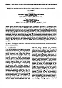
Figure 2: Object Handling differencing scheme described below. The differencing scheme we use stores only the difference between the descriptions of a child node and its parent. In other words, given a node, we store a relative description that has the newly added objects, removed objects and changed objects compared with its parent. For the root of a subtree, the differencing scheme always stores an explicit description consisting of all the objects active at the root. To store a relative description for a node, the differencing scheme identifies the relative difference of this node with its parent. The data structures used to record differences are BcpsFieldListMod and BcpsObjectListMod. The class BcpsFieldListMod stores the modifications in single field, such as the lower bounds of the variables, for example. The class BcpsObjectListMod, on the other hand, stores modifications of the overall lists of variables and constraints active in the node. A flag can be set to indicate that explicit storage of the node is more efficient than storing the difference data. Note that our differencing scheme for storing the search tree also means that the we may have to spend time simply recovering the explicit description of tree nodes. This is done by working down the tree from the first ancestor with an explicit description applying the differences until an explicit description of the node is obtained. This is the trade-off between saving space and increasing search time. To prevent too much time being spent in recovering node descriptions, the differencing scheme has the option to force storage of an explicit description for all nodes at a certain depth below the last explicitly stored description. 3.2.2
Task Management
BiCePS assumes that the algorithm employs an iterative bounding scheme. During each iteration, new objects may be generated and used to improve the fidelity of the current relaxation. Because the number of objects generated in each iteration may be quite large, newly generated objects may first be placed in a local pool that acts as a cache of potential candidates for addition. Duplicate and ineffective objects previously added to the relaxation are generally removed aggressively in order to control the size of the relaxation. Those that prove to be particularly effective may be added to a global pool for sharing with other KBs. Figure 2 shows the object handling scheme of BiCePS pictorially.
11
3.3 3.3.1
BLIS Knowledge Management.
The BLIS library provides the functionality needed to solve mixed integer linear programs and consists mainly of classes derived from BiCePS with a few additions. The class names in Figure 1 with prefix Blis belong to BLIS library. BLIS has classes BlisConstraint, BlisVariable, BlisSolution, BlisTreeNode, BlisNodeDesc, and BlisModel, all derived from the classes in BiCePS. Other classes include those for specifying algorithms for constraint generation, primal heuristics, and branching strategies. In the next few section, we briefly overview the types of knowledge that must be shared in BLIS. Note that some knowledge types, such as bounds and pseudo-costs are not treated as abstract knowledge types because of their simple structure and sharing mechanisms. Bounds. The bounds that must be shared in branch and cut consist of the single global upper bound and the lower bounds associated with the subproblems that are candidates for processing. Knowledge of lower bounds is important mainly for load balancing purposes and is shared according to the scheme described in Section 3.1.3. Distribution of information regarding upper bounds is mainly important for avoiding performance of redundant work, i.e., processing of nodes whose lower bound is above the optimal value. Distribution of this information is relatively easy to handle because relatively few changes in upper bound typically occur throughout the algorithm. Branching Information. If a backward-looking branching method, such as one based on pseudocosts, is used, then the sharing of historical information regarding the effect of branching can be important to the implementation of the branching scheme. The information that needs to be shared and how it is shared depends on the specific scheme used. For an in-depth treatment of the issues surrounding pseudo-cost sharing in parallel, see [11] and [31]. Variables and Constraints. One of the advantages of branch and cut over generic LP-based branch and bound is that the inequalities generated at each node of the search tree may be valid and useful in the processing of search tree nodes in other parts of the tree. Valid inequalities are usually categorized as either globally valid (valid for the convex hull of solutions to the original MILP and hence for all other subproblems as well), or locally valid (valid only for the convex hull of solutions to a given subproblem). Because some classes of valid inequalities are difficult to generate, inequalities that prove effective in the current subproblem may be shared through the use of cut pools that contain lists of such inequalities for use during the processing of subsequent subproblems. The cut pools can thus be utilized as an auxiliary method of generating violated valid inequalities during the processing operation. 3.3.2
Task Management
In branch and cut, there are a number of distinct tasks to be performed and these tasks can be assigned to processors in a number of ways. The main tasks to be performed are: • Node processing: From the description of a candidate node, the processing procedure produces either an improved bound or a feasible solution to the original MILP. 12
• Node partitioning: From the description of a processed node, the partitioning procedure is used to select a method of branching and subsequently produce a set of children to be added to the candidate list. • Cut generation: From a solution to a given LP relaxation produced during node processing, the cut generation procedure produces a violated valid inequality (either locally or globally valid). • Pool maintenance: Some processors may be assigned the task of managing either node or cut pools. • Load balancing: One or more processors may be assigned the task of collecting information about the distribution of candidate subproblems globally and coordinating their redistribution when necessary (see Section 3.1.3). The way in which these tasks are grouped and assigned to processors determines, to a large extent, the parallelization scheme of the algorithm and its scalability. In the current implementation of BLIS, node processing, cut generation, and node partitioning are all handled locally during processing of each subtree. Load balancing is handled as previously described. Branching. The branching scheme of BLIS is similar to that of the COIN-OR Branch and Cut framework (CBC) [14] and comprises three components: • Branching Objects: BiCePS objects that can be branched on, such as integer variables and SOS sets. • Candidate Branching Objects: Objects that do not lie in the feasible region or objects that will be beneficial to the search if branching on them. • Branching Method : A method to compare objects and choose the best one. The branching method is a core component of BLIS’s branching scheme. When expanding a node, the branching method first identifies a set of initial candidates and then selects the best object based on the rules it specifies. Figure 3 shows the major steps of BLIS’s branching scheme. The branching methods provided by BLIS include strong branching, pseudo-cost branching, reliability branching and maximum infeasibility branching. Users can develop their own branching methods by deriving subclasses from BcpsBranchStrategy. Constraint Generation. BLIS constraint generators are used to generate additional constraints to improve problem formulation. BLIS constraint generators have methods to collect statistics that can be used to manage constraint generation. Users have the ability to specify rules to control a generator: • where to call the generator? • how many constraints can the generator generate at most? • when to activate or disable the generator? 13
Figure 3: Branching Scheme
Figure 4: Constraint Generator As Figure 4 shows, BLIS stores the generated constraints in local constraint pools. Later, BLIS augments the current subproblem with some or all of the newly generated constraints. The BLIS constraint generator base class also provides an interface between BLIS and the algorithms in the COIN-OR Cut Generator Library (CGL). Therefore, BLIS can use all the constraint generators in CGL, a library of cut generation methods. Users can develop CGL constraint generators or derive generators from the BLIS constraint generator base class, and then add them into BLIS. Primal Heuristics. The BLIS primal heuristic class declares the methods needed to search heuristically for feasible solutions. The class also provides the ability to specify rules to control the heuristic, such as • where to call the heuristic? • how often to call the heuristic? • when to activate or disable the heuristic? The methods in the class collect statistics to guide searching and provides a base class for deriving various heuristics. Currently, BLIS has only a simple rounding heuristic.
14
4
Computation
We conducted a number of experiments to test the performance of the methodology described above in order to identify the major contributors to parallel overhead and the effectiveness of our attempts to improve scalability across a wide range of MILP instances. All tests were performed on a Beowulf cluster at Clemson University and a Blue Gene system at the San Diego Supercomputer Center (SDSC) [46]. The Clemson cluster has 52 nodes, each with a dual-core IBM Power5 PPC64 chip. The core speed is 1654 MHz. The two cores share 4 GB RAM, as well as L2 and L3 cache, but have their own L1 cache. The Blue Gene system has three racks with 3072 compute nodes and 384 I/O nodes. Each compute node consists of two PowerPC processors that run at 700 MHz and share 512 MB of memory. In Sections 4.1, we first analyze the overall scalability of CHiPPS with default parameter settings. In Sections 4.2, we report on tests of the individual effectiveness of various schemes to improve scalability, including the master-hub-worker paradigm, the load balancing schemes, and the differencing scheme. It should be noted that the challenges that arise in testing a parallel implementation like this one are many and difficult to overcome. For this reason, results such as those presented here have always to be taken with a healthy degree of skepticism because the amount of variability in experimental conditions is such that it is often extremely difficult to tease out the exact causes for observed behavior. The situation is even more difficult when it comes to providing comparisons to other implementations. This is in part because the scalability properties of individual instances can be very different under different conditions, making it difficult to choose a test set that is simultaneously appropriate for multiple solvers. We have done our best to provide some basis for comparison in the results below, but this is ultimately a very difficult task.
4.1
Overall Scalability
We first report results of solving knapsack instances with a simple knapsack solver that we refer to below as KNAP, which was built directly on top of ALPS. This solver uses a straightforward branch-and-bound algorithm with no cut generation. These experiments allowed us to look independently at aspects of our framework having to do with the general search strategy, load balancing mechanism, and the task management paradigm. We tested KNAP using two different test sets, one composed of moderately difficult instances and the other composed of much more difficult instances. Finally, we report results of solving a set of generic MILPs with BLIS and discuss the impact of the properties of individual instances on scalability. 4.1.1
Solving Moderately Difficult Knapsack Instances
We randomly generated 10 moderately difficult knapsack instances based on the method proposed by Martello and Toth [34]. We tested these ten instances by using 4, 8, 16, 32, and 64 processors (cores) on the Clemson cluster. These instances are difficult to solve when using the sequential version of KNAP because the number of nodes that must be enumerated is very large and memory becomes an issue. They can all be solved to optimality quite easily, however, with as few as 4 processors. Because the results of the ten instances show a similar pattern, we aggregated the results, which are shown in Table 1. The column headers have the following interpretations: 15
Table 1: Scalability for Solving Moderately Difficult Knapsack Instances P 4 8 16 32 64
Nodes 193057493 192831731 192255612 191967386 190343944
Ramp-up 0.28% 0.58% 1.20% 2.34% 4.37%
Idle 0.02% 0.08% 0.26% 0.71% 2.27%
Ramp-down 0.01% 0.09% 0.37% 1.47% 5.49%
Wallclock 586.90 245.42 113.43 56.39 30.44
Eff 1.00 1.20 1.29 1.30 1.21
• Nodes is the number of nodes in the search tree. Observing the change in the size of the search tree as the number of processors is increased provides a rough measure of the amount of redundant work being done. Ideally, the total number of nodes explored does not grow as the number of processors is increased and may actually decrease in some cases, due to earlier discovery of feasible solutions that enable more effective pruning. • Ramp-up is the average percentage of total wallclock running time time each processor spent idle during the ramp-up phase. • Idle is the average percentage of total wallclock running time each processor spent idle due to work depletion during the primary phase of the algorithm. • Ramp-down is the average percentage of total wallclock running time time each processor spent idle during the ramp-down phase. • Wallclock is the total wallclock running time (in seconds) for solving the 10 knapsack instances. • Eff is the parallel efficiency and is equal to the total wallclock running time for solving the 10 instances with p processors divided by the product of 4 and the total running time with four processor. Note that the efficiency is being measured here with respect the solution time on four processors, rather than one, because of the memory issues encountered in the single-processor runs. Efficiency should normally represent approximately the average fraction of time spent by processors doing “useful work,” where the amount of useful work to be done, in this case, is measured by the running time with four processors. Efficiencies greater than one are not typically observed and when they are observed, they are usually the result of random fluctuations or earlier discovery of good incumbents. Here we observe that the total number of nodes remains relatively constant, so the so-called “superlinear speedup” observed may again be due to minor memory issues encountered in the four processor runs. In any case, it can be observed that the overhead due to ramp-up, ramp-down, and idle time remains low as the number of processors is scaled up. Other sources of parallel overhead were not measured directly, but we can easily infer that these sources of overhead are negligible. 4.1.2
Solving Difficult Knapsack Instances
We further tested the scalability of ALPS by using KNAP to solve 26 very difficult knapsack instances, which were also generated based on the method proposed by Martello and Toth [34]. This 16
Table 2: Scalability for Solving Difficult Knapsack Instances P 64 128 256 512 1024 2048
Nodes 14733745123 14776745744 14039728320 13533948496 13596979694 14045428590
Ramp-up 0.69% 1.37% 2.50% 7.38% 13.33% 9.59%
Idle 4.78% 6.57% 7.14% 4.30% 3.41% 3.54%
Ramp-down 2.65% 5.26% 9.97% 14.83% 16.14% 22.00%
Wallclock 6296.49 3290.56 1672.85 877.54 469.78 256.22
Eff 1.00 0.95 0.94 0.90 0.84 0.77
experiment was conducted on the SDSC Blue Gene system. Table 2 shows the aggregated results. For this test, we used the time for the 64-processor run as our baseline for measuring efficiency. The experiment shows that KNAP scales well, even when using several thousand processors. This is because the node evaluation times are generally short and it is easy to generate a large number of nodes quickly during ramp-up. For this reason, the workload is already quite well balanced at the beginning of the search. As the number of processors is increased to 2048, we observe that the wallclock running time of the main phase of the algorithm becomes shorter and shorter, while the running time of the ramp-up and ramp-down phases inevitably increase, with these phases eventually dominating the overall wallclock running time. This is an example of the phenomenon described earlier in Section 2 whereby the inherently sequential portions of the algorithm limit the overall scalability of a fixed set of test instances. To get a truer picture of how the algorithm scales beyond the current 2048 processors, we would need to scale the size and difficulty of the instances while scaling the number of processors, as suggested by Kumar and Rao [27]. This analysis was not performed due to resource limitations and the practical difficulty of constructing appropriate test sets. 4.1.3
Solving Generic MILPs
We selected 18 MILP instances from Lehigh/CORAL, MIPLIB 3.0, MIPLIB 2003 [1], BCOL [6], and [33]. These instances took at least two minutes but no more than 2 hours to solve with BLIS sequentially. We used four cut generators from the COIN-OR Cut Generation Library [14]: CglGomory, CglKnapsackCover, CglFlowCover, and CglMixedIntegerRounding. Pseudocost branching was used to select branching objects. The local search strategy was a hybrid diving strategy in which one of the children of a given node was retained as long as its bound did not exceed the best available by more than a given threshold. As per default parameter settings, ALPS used two hubs for the runs with 64 processors. For all other runs, one hub was used. Table 3 shows the results of these computations. Note that in this table, we have added an extra column to capture sources of overhead other than idle time (i.e., communication overhead) because these become significant here. The effect of these sources of overhead is not measured directly, but must be estimated as the difference between the efficiency and the fraction of time attributed to the other three sources. Note also that in these experiments, the master process does not do any exploration of subtrees, so an efficiency of (p − 1)/p is the best that can be expected, barring anomalous behavior. To solve these instances, BLIS needed to process a relatively large number of nodes and the node processing time were generally not long. These two properties tend to lead
17
Table 3: Scalability for generic MILP Instance 1P Per Node 4P Per Node 8P Per Node 16P Per Node 32P Per Node 64P Per Node
Nodes 11809956 11069710 11547210 12082266 12411902 14616292
Ramp -up − − 0.03% 0.03% 0.11% 0.14% 0.33% 0.27% 1.15% 1.22% 1.33% 1.38%
Idle − − 4.62% 4.66% 4.53% 4.52% 5.61% 5.66% 8.69% 8.78% 11.40% 11.46%
Ramp -down − − 0.02% 0.02% 0.41% 0.53% 1.60% 1.62% 2.95% 2.93% 6.70% 6.72%
Comm Overhead − − 16.33% 16.34% 16.95% 16.95% 17.46% 17.45% 21.21% 21.07% 34.57% 34.44%
Wallclock
Eff
33820.53 0.00286 10698.69 0.00386 5428.47 0.00376 2803.84 0.00371 1591.22 0.00410 1155.31 0.00506
1.00 0.79 0.78 0.75 0.66 0.46
to good scalability and the results reflect this to a large extent. However, as expected, overhead starts to dominate wallclock running time across the board as the number of processors is increased. This is again an example of the limitations in scalability of a fixed test predicted by Amdahl (see Section 2). Examining each component of overhead in detail, we see that ramp-up, idle, and ramp-down time grow, as a percentage of overall running time, as the number of processors increases. This is to be expected and is in line with the performance seen for the knapsack problems. However, the communication overhead turns out to be the major cause of reduced efficiency. We suspect this is for two reasons. First, the addition of cut generation increases the size of the node descriptions and the amount of communication required to do the load balancing. Second, we found that as the number of processors increased, the amount of load balancing necessary went up quite dramatically, in part due to the ineffectiveness of the static load balancing method for these problems. Table 4 summarizes the aggregated results of load balancing and subtree sharing when solving the 18 instances that were used in the scalability experiment. The column labeled P is the number of processors. The column labeled Inter is the number of inter-cluster balancing operations performed (this is zero when only one hub is used). The column labeled Intra is the number of intra-cluster balancing operations performed. The column labeled Starved is the number of times that workers reported being out of work and proactively requested more. The column labeled Subtree is the number of subtrees shared. The column labeled Split is the number of subtrees that were too large to be packed into a single message buffer and had to be split when sharing. The column labeled Whole is the number of subtrees that did not need to be split. As Table 4 shows, the total number of inter- and intra-cluster load balancing operations goes down when the number of processors increases. However, worker starvation increases. Additionally, the number of subtrees needing to be split into multiple message units increases. These combined effects seem to be the cause of the increase in communication overhead. In order to put these results in context, we have attempted to analyze how they compare to results reported in papers in the literature, of which there are few. Eckstein et al. tested the scalability of 18
Table 4: Load Balancing and Subtrees Sharing P 4 8 16 32 64
Inter 0 0 0 0 494
Intra 87083 37478 15233 7318 3679
Starved 22126 25636 38115 44782 54719
Subtree 42098 41456 55167 59573 69451
Split 28017 31017 44941 50495 60239
Whole 14081 10439 10226 9078 9212
PICO [11] by solving 6 MILP instances from MIPLIB 3.0. For these tests, PICO was used as a pure branch and bound code and did not have any constraint generation, so it is difficult to do direct comparison. One would expect that the lack of cut generation would increase the size of the search tree while decreasing the node processing time, thereby improving scalability. Their experiment showed an efficiency 0.73 for 4 processors, 0.83 for 8 processors, 0.69 for 16 processors, 0.65 for 32 processors, 0.46 for 64 processors, and 0.25 for 128 processors. Ralphs [38] reported that the efficiency of SYMPHONY 5.1 is 0.81 for 5 processors, 0.89 for 9 processors, 0.88 for 17 processors, and 0.73 for 33 processors when solving 22 MILP instances from Lehigh/CORAL, MIPLIB 3.0, and MIPLIB 2003. All in all, our results are similar to those of both PICO and SYMPHONY. However, because we are using a more sophisticated and therefore less scalable algorithm, this can be seen as an improvement. Also, SYMPHONY was not tested beyond 32 processors and it is unlikely that it would have scaled well beyond that. In the next section, we show this by comparing the performance of BLIS and SYMPHONY when solving knapsack problem. 4.1.4
Comparison of BLIS and SYMPHONY
As we have already described, it is not straightforward to compare the performance of two parallel solvers, in part because of the fact that it is difficult to find a set of test instances appropriate for testing both solvers simultaneously. Ralphs [38] reported that SYMPHONY is very effective for small number of processors, but is not scalable well beyond about 32 processors. To see how BLIS compares to SYMPHONY, we randomly generated 10 knapsack instances based on the method proposed by Martello and Toth [34]. The experiment was performed on the Clemson cluster, and the default settings of BLIS and SYMPHONY were used. Note that for these experiments, we used BLIS, including full cut generation, not the KNAP application discussed above. The aggregated results are summarized in Table 5. Column P is the number of processors. Column Solver is the solver used. The other columns have the same meaning as those in Table 3. It can be seen from these results that BLIS scales reasonably well and the overhead is relatively small. However, SYMPHONY has trouble scaling as the number processors increase because it suffers from a number of synchronization bottlenecks, mainly as a result of the fact that many workers are being controlled by a single master. In SYMPHONY, the task granularity is also much smaller (fixed at one node). The effect of this is seen in the results here, as the efficiency is already extremely low with just 16 processors. BLIS also begins to show efficiency degradation when using 16 processors, but this is mainly due to the fact that these problems are too easy and Amdahl’s law is coming into play, as discussed earlier. As a side note, BLIS appears to be much more effective on these instances than SYMPHONY—we suspect this is due to SYMPHONY’s inferior cut generation strategy.
19
Table 5: Scalability of BLIS and SYMPHONY for Knapsack Instances P 1 4 8 16
4.1.5
Solver BLIS SYM BLIS SYM BLIS SYM BLIS SYM
Nodes 450644 5465932 435990 4935156 347126 4944232 369586 4957982
Ramp-up − − 0.08% 0.01% 0.30% 0.49% 0.77% 0.16%
Idle − − 3.16% 28.40% 4.74% 42.92% 8.00% 62.77%
Ramp-down − − 2.46% 0.12% 6.37% 1.73% 18.32% 3.78%
Wallclock 124.67 3205.77 38.63 1659.55 16.65 1070.03 10.37 847.43
Eff 1.00 1.00 0.80 0.48 0.94 0.37 0.75 0.23
The Impact of Problem Properties
As we have mentioned several times, the properties of individual instances can significantly affect scalability, independent of the implementation of the solver itself. Table 6 shows the detailed results of solving three specific MILP instances with BLIS. The tests were performed on SDSC Blue Gene. We use the time for the 64-processor run as the baseline for measuring efficiency. Instance input150 1 is a knapsack instance. When using 128 processors, BLIS achieved superlinear speedup mainly due to the decrease in the tree size. BLIS showed good parallel efficiency as the number processors increase to 256 and 512. Instance fc 30 50 2 is a fixed-charge network flow instance. It exhibits very significant increases in the size of its search tree (indicating the performance of redundant work) as the number of processors increases, resulting in decreased efficiency. It was found that the optimality gap of instancefc 30 50 2 improves very slowly during the search, which causes a large number of node to be processed. Instance pk1 is a small integer program with 86 variables and 45 constraints. It is relatively easy to solve. Although the efficiency is reasonable good when using 128 processors, it is eventually wiped out by significant increases in ramp-up and ramp-down overhead as the number of processors increases. The results in Table 6 show that problem properties can have a tremendous impact on scalability. For instances that have large tree size and short node processing time, it is not difficult to achieve good speedup. For instances that are particularly easy to solve or for which the upper bounds are difficult to improve, however, it can be difficult to achieve good speedup regardless of the effectiveness of the implementation.
4.2
The Effectiveness of the Schemes for Performance Improvement
As discussed before, CHiPPS employs a number of schemes to improve performance. We conducted several experiments to verify the effectiveness of those schemes are. In this section, we report the results of these experiments.
20
Table 6: Problem Properties and Scalability Instance input150 1
fc 30 50 2
pk1
P 64 128 256 512 64 128 256 512 64 128 256 512
Node 75723835 64257131 84342537 71779511 3494056 3733703 6523893 13358819 2329865 2336213 2605461 3805593
Ramp-up 0.44% 1.18% 1.62% 3.81% 0.15% 0.22% 0.23% 0.27% 3.97% 11.66% 11.55% 19.14%
Idle 3.38% 6.90% 5.53% 10.26% 31.46% 33.25% 29.99% 23.54% 12.00% 12.38% 13.93% 9.07%
Ramp-down 1.45% 2.88% 7.02% 10.57% 9.18% 21.71% 28.99% 29.00% 5.86% 10.47% 20.19% 26.71%
Wallclock 1257.82 559.80 380.95 179.48 564.20 399.60 390.12 337.85 103.55 61.31 41.04 36.43
Eff 1.00 1.12 0.83 0.88 1.00 0.71 0.36 0.21 1.00 0.84 0.63 0.36
Table 7: Effect of Master-hub-worker Paradigm Hubs 1 2 4 8 16 32 64 128
4.2.1
Cluster Size 1024 512 256 128 64 32 16 8
Node 2189900404 2181608684 2671387391 2138187406 2132342280 2132560921 2136262257 2150789246
Ramp-up 14.78% 16.43% 18.76% 20.45% 22.38% 22.61% 20.38% 14.69%
Idle 2.25% 4.04% 3.17% 2.57% 1.71% 1.04% 0.75% 0.85%
Ramp-down 38.17% 29.64% 18.13% 17.27% 11.99% 11.17% 13.78% 14.12%
Wallclock 103.79 91.74 91.10 74.57 70.14 71.44 82.13 118.31
The Master-Hub-Worker Paradigm
An important aspect of the scheme for scalability improvement in ALPS is the implementation of the master-hub-worker paradigm. By adding the hubs in between the master and the workers, we hoped that parallel overhead can be reduced. In this test, we examine whether using hubs does actually help to improve performance. The test was conducted on the SDSC Blue Gene system. We used the moderately difficult knapsack instance set and ran KNAP on 1024 processors. Table 7 shows the aggregated results using 1, 2, 4, 8, 16, 32, 64 and 128 processors. The column labeled Hubs is the number of hubs used. Column ClusterSize is the number of processes in each cluster. From the table, we can see that the use of multiple hubs does improve efficiency as long as the cluster size is not too small. In particular, we see that the hubs have a difficult time balancing the workload of workers at the end of the search if the number of hubs used is small and the master has a difficult time balancing the workload among the clusters if the number of hubs is large. For this test, a cluster size of 32 or 64 seems to be optimal.
21
Table 8: Effect of Intra-cluster Load Balancing P 64 128
Intra Yes No Yes No
Node 190343944 190344811 190885657 190932329
Ramp-up 4.37% 3.38% 7.84% 6.38%
Idle 2.27% 0.00% 3.97% 0.00%
Ramp-down 5.49% 28.06% 10.14% 30.59%
Wallclock 30.44 39.35 19.14 23.18
Table 9: Effect of inter-cluster Load Balancing Hubs 16 32 64 128
4.2.2
Inter Yes No Yes No Yes No Yes No
Node 2132342280 2131879616 2132560921 2131980156 2136262257 2136236456 2150789246 2149541063
Ramp-up 22.38% 22.52% 22.61% 22.43% 20.38% 20.35% 14.69% 14.62%
Idle 1.71% 1.73% 1.04% 0.90% 0.75% 0.40% 0.85% 0.17%
Ramp-down 11.99% 11.57% 11.17% 12.07% 13.78% 14.33% 14.12% 15.33%
Wallclock 70.14 69.85 71.44 72.01 82.13 82.34 118.31 119.01
Intra-cluster Dynamic Load Balance
We tested the effect of the intra-cluster load balancing by comparing the results obtained with and without the dynamic load balancing schemes. For this experiment, we used one hub and solved the ten moderately difficult knapsack instances with KNAP on 64 and 128 processors. The experiment was conducted on the Clemson cluster. Table 8 presents the aggregated results of the ten instances. A Yes in the second column indicates that the intra-cluster dynamic load balancing was turned on, and a No means it was turned off. The results demonstrate that the load balancing scheme is very important in maintaining scalability. Without dynamic load balancing, the wallclock running time increases substantially. Furthermore, knapsack examples tend to be very well behaved with respect to the effect of the initial static load balancing. this indicates that the effect would be even more pronounced for other types of MILP instances. 4.2.3
Inter-cluster Dynamic Load Balance
In this experiment, we wanted to check the effect of the inter-cluster load balancing. The test was conducted on the SDSC Blue Gene system. We solved the ten moderately difficult knapsack instances with KNAP, and used 1024 processors. We compared the results using the inter-cluster dynamic load balancing with those not using it. Table 9 presents the aggregated results of the ten instances. The column labeled Hubs indicates how many hubs were used. A Yes in the second column means the inter-cluster dynamic load balancing was turned on, and a No means it was turned off. The results show that for this test set, parallel efficiency does not change much when inter-cluster dynamic load balancing is turned on. However, we suspect that this is because the static load balancing scheme works particularly well for these relatively well behaved instances. 22
4.2.4
Differencing
To test the differencing scheme, we chose 38 MILP instances from the Lehigh/COR@L [30] and MIPLIB 3.0 [2] test sets that can be solved by BLIS serially within a 10 minute time limit. We solved each instance with and without using the differencing scheme and measured the peak memory requirement in each case. Overall, the runs with the differencing scheme exhibited an 80% reduction in peak memory requirements. In addition, the running time was slightly faster when employing the differencing scheme, a result that was quite pleasantly surprising. In parallel, the scheme should also result in reductions in the communication overhead due to smaller message sizes. On the whole, the differencing scheme seems to be quite effective.
5
Conclusions and Future Work
In this paper, we have introduced the basic concepts and methodology required for parallelization of relaxation-based branch-and-bound algorithms, particularly the well-known branch-and-cut algorithm. Parallelizing such algorithms in a scalable fashion is a challenge that involves balancing the costs and benefits of synchronization and the sharing of knowledge during the algorithm. Because this analysis can yield different results for different problem classes, it is difficult in general to develop a single ideal approach that will be effective across all problem classes. However, the asynchronous and decentralized approach taken by CHiPPS has proven to be effective across a fairly wide range of instances. Nevertheless, many challenges remain. In the near term, we plan to continue improving CHiPPS by refining the load balancing schemes and knowledge sharing methods. Reducing the length of the ramp-up and ramp-down phases will be a particular focus, as effort during these phases remains a significant scalability issue. We also plan to generalize the current implementation of BLIS in order to better support column generation and related algorithms, such as branch and price. In the longer term, we are planning to develop additional modules for solution of additional problem classes, such as non-linear programs. We also hope to improve fault tolerance and develop a knowledge broker appropriate for deployment on computational grids.
References [1] MIPLIB 2003. http://miplib.zib.de. [2] MIPLIB 3. htpp://www.caam.rice.edu/ bixby/miplib/miplib3.html. [3] G.M. Amdahl. Validity of the single-processor approach to achieving large-scale computing capabilities. In AFIPS Conference Proceedings, pages 483–485. AFIPS Press, 1967. [4] D. Applegate, R. Bixby, V. Chv´atal, and W. Cook. www.keck.caam.rice.edu/concorde.html.
CONCORDE TSP solver.
[5] D. Applegate, R. Bixby, V. Chv´atal, and W. Cook. On the solution of traveling salesman problems. Documenta Mathematica, Extra Volume Proceedings ICM III (1998):645–656, 1998. [6] Berkeley Computational Optimization Lab (BCOL). ~atamturk/bcol.
23
http://www.ieor.berkeley.edu/
[7] M. Benchouche, V.-D. Cung, S. Dowaji, B. Le Cun, T. Mautor, and C. Roucairol. Building a parallel branch and bound library. In Solving Combinatorial Optimization Problems in Parallel, Lecture Notes in Computer Science 1054. Springer, Berlin, 1996. [8] B. Borbeau, T.G. Crainic, and B. Gendron. Branch-and-bound parallelization strategies applied to a depot location and container fleet management problem. Parallel Computing, 26:27– 46, 2000. [9] R.G. Brown. Engineering a beowulf-style compute cluster. Available from http://www.phy. duke.edu/~rgb/Beowulf/beowulf_book/beowulf_book/, 2004. [10] Q. Chen and M. Ferris. Fatcop: A fault tolerant condor-pvm mixed integer programming solver. SIAM Journal on Optimization, 11(4):1019–1036, 2001. [11] J. Eckstein, C.A. Phillips, and W.E. Hart. Pico: An object-oriented framework for parallel branch and bound. Technical Report RRR 40-2000, Rutgers University, 2000. [12] J. Eckstein, C.A. Phillips, and W.E. Hart. Pebbl 1.0 user guide, 2007. [13] C. Fonlupt, P. Marquet, and J. Dekeyser. Data-parallel load balancing strategies. Parallel Computing, 24(11):1665–1684, 1998. [14] Computational Infrastructure for Operations Research. http://www.coin-or.org. [15] Al Geist, Adam Beguelin, Jack Dongarra, Weicheng Jiang, Robert Manchek, and Vaidyalingam S. Sunderam. PVM: Parallel Virtual Machine: A Users’ Guide and Tutorial for Networked Parallel Computing. MIT Press, Cambridge, MA, USA, 1994. [16] B. Gendron and T. G. Crainic. Parallel branch and bound algorithms: Survey and synthesis. Operations Research, 42:1042–1066, 1994. [17] B. Gendron, T.G. Crainic, A. Frangioni, and F. Guertin. Oobb: Object-oriented tools for parallel branch-and-bound, 2005. [18] A.Y. Grama and V. Kumar. Parallel search algorithms for discrete optimization problems. ORSA Journal on Computing, 7:365–385, 1995. [19] W. Gropp, E. Lusk, and A. Skjellum. Using MPI. MIT Press, Cambridge, MA, USA, 2nd edition, 1999. [20] J.L. Gustafson. Reevaluate amdahl’s law. Comm. ACM, 31(1):532–533, 1988. [21] L. Hafer. bonsaiG: Algorithms and design. Technical Report TR 1999-06, 1999. [22] D. Henrich. Initialization of parallel branch-and-bound algorithms. In Second International Workshop on Parallel Processing for Artificial Intelligence(PPAI-93), August, 1993. [23] M. J¨ unger and S. Thienel. The abacus system for branch and cut and price algorithms in integer programming and combinatorial optimization. Software Practice and Experience, 30:1325– 1352, 2001. [24] GNU Linear Programming Kit. http://www.gnu.org/software/glpk. [25] V. Kumar, A.Y. Grama, and Nageshwara Rao Vempaty. Scalable load balancing techniques for parallel computers. Journal of Parallel and Distributed Computing, 22(1):60–79, 1994. 24
[26] V. Kumar and A. Gupta. Analyzing scalability of parallel algorithms and architectures. Journal of Parallel and Distributed Computing, 22:379–391, September 1994. [27] V. Kumar and V. N. Rao. Parallel depth-first search, part II: Analysis. International Journal of Parallel Programming, 16:501–519, 1987. [28] A.H. Land and A.G. Doig. An automatic method for solving discrete programming problems. Econometrica, 28:497–520, 1960. [29] P.S. Laursen. Can parallel branch and bound without communication be effective? SIAM Journal on Optimization, 4:33–33, May, 1994. [30] Lehigh/CORAL. http://coral.ie.lehigh.edu. [31] J. Linderoth. Topics in Parallel Integer Optimization. PhD thesis, School of Industrial and Systems Engineering, Georgia Institute of Technology, Atlanta, GA, 1998. [32] lpsolve. http://tech.groups.yahoo.com/group/lpsolve. [33] markshare. http://miplib.zib.de/contrib/Markshare. [34] S. Martello and P. Toth. Knapsack Problems: Algorithms and Computer Implementation. John Wiley & Sons, Inc., USA, 1st edition, 1990. [35] L.G. Mitten. Branch-and-bound methods: General formulation and properties. Operations Research, 18:24–34, 1970. [36] G. L. Nemhauser, M.W.P. Savelsbergh, and G.S. Sigismondi. Minto, a mixed integer optimizer. Operations Research Letters, 15:47–58, 1994. [37] G.L. Nemhauser and L.A. Wolsey. Integer and Combinatorial Optimization. John Wiley & Sons, Inc., USA, 1st edition, 1988. [38] T. K. Ralphs. Parallel branch and cut. In E. Talbi, editor, Parallel Combinatorial Optimization. Wiley, USA, 2006. [39] T. K. Ralphs, L. Lad´ anyi, and M. J. Saltzman. Parallel branch, cut, and price for large-scale discrete optimization. Mathematical Programming, 98:253–280, 2003. [40] T.K. Ralphs and L. Lad´ anyi. COIN/BCP User’s Manual, 2001. Available from http://www. coin-or.org. [41] T.K. Ralphs and L. Lad´ anyi. SYMPHONY Version 5.0 User’s Manual, 2005. http://www. brandandcut.org. [42] T.K. Ralphs, L. Lad´ anyi, and M.J. Saltzman. A library hierarchy for implementing scalable parallel search algorithms. The Journal of Supercomputing, 28:215–234, 2004. [43] P. Sanders. Tree shaped computations as a model for parallel applications, 1998. [44] Y. Shinano, K. Harada, and R. Hirabayashi. A generalized utility for parallel branch and bound algorithms. In Proceedings of the 1995 Seventh Symposium on Parallel and Distributed Processing, pages 392–401, Los Alamitos, CA, 1995. IEEE Computer Society Press.
25
[45] A. Sinha and L.V. Kal´e. A load balancing strategy for prioritized execution of tasks. In Seventh International Parallel Processing Symposium, pages 230–237, Newport Beach, CA., April 1993. [46] TeraGrid. http://www.teragrid.org. [47] H. W. J. M. Trienekens and A. De Bruin. Towards a taxonomy of parallel branch and bound algorithms. Technical Report EUR-CS-92-01, Department of Computer Science, Erasmus University, 1992. [48] S. Tschoke and T. Polzer. Portable Parallel Branch and Bound Library User Manual: Library Version 2.0. Department of Computer Science, University of Paderborn. [49] Y. Xu, T.K. Ralphs, L. Lad´ anyi, and M.J. Saltzman. ALPS: A framework for implementing parallel search algorithms. In Proceedings of the Ninth INFORMS Computing Society Conference, pages 319–334, 2005.
26