Artificial Neural Networks - Advances in Computational Intelligence and Learning. Bruges (Belgium), 23-25 April 2008, d-side publi., ISBN 2-930307-08-0.
ESANN'2008 proceedings, European Symposium on Artificial Neural Networks - Advances in Computational Intelligence and Learning Bruges (Belgium), 23-25 April 2008, d-side publi., ISBN 2-930307-08-0.
Computational Model for Amygdala Neural Networks Jean Marc Salotti 1- Laboratoire Cognition et Facteurs Humains, Institut de Cognitique, Université de Bordeaux IDC, 146 Rue Léo Saignat, 33076 Bordeaux Cedex - France Abstract. We present a computational model of amygdala neural networks. It is used to simulate neuronal activation in amygdala nuclei at different stages of aversive conditioning experiments with rats. Our model is based on neurobiological data. Simple formal neurons and an adaptive Hebbian rule are the key elements of the model. The results are compatible with neuronal activation maps obtained with C-Fos markers. The model also enables interesting predictions.
1
Introduction
In order to better understand the role of amygdala nuclei in drug addiction and weaning treatments, aversive experiments have been conducted with rats. A box with three compartments is used. Before experiments, rats are addicted to morphine. In the first stage, a rat is left in the first compartment without access to the others and a naloxone injection is undergone. During a few minutes, its moves become slow and awkward. The same experiment is repeated three times during a period of six days. Then, it is simply placed in the box and its behavior is observed. The rat tends to avoid the compartment in which it underwent the naloxone injection, thus proving the set up of an aversive conditioning. Since the role of amygdala nuclei is well known in aversive conditioning experiments, neuronal activity maps of that part of the brain have been obtained at different moments. We distinguish between two important nuclei of the amygdaloid complex: the basolateral one (BlA) and the central one (CeA). These maps are presented Figure 1. Many details of the experiments that have been conducted are not presented here. The reader can get more information from previous publications [2]. The problem we want to discuss here is the way we can determine and implement a computational model of the amygdala nuclei with sufficient details, so that it explains what is observed and it can be predictive for other experiments. In Section 2, we present different approaches in computational neuroscience and discuss the methodology that should be used for that problem. In Section 3, we give the specifications of the computational model and present our network. We finally provide some results in Section 4 and discuss the perspectives.
2
Methodology
In computational neuroscience, Perkel propose to distinguish among six different levels, according to the scale and the dynamics at which the problem is addressed [4]. The first levels are concerned with molecular chemistry and the study of dendrites, axons, synapses, or the dynamics of few neurons.
403
ESANN'2008 proceedings, European Symposium on Artificial Neural Networks - Advances in Computational Intelligence and Learning Bruges (Belgium), 23-25 April 2008, d-side publi., ISBN 2-930307-08-0.
Fig. 1: Left, just after the first naloxone injection, the CeA is strongly activated. Middle, during the aversive conditioning test, the CeA is poorly activated, while the BlA is more activated. Right, the activity map of a control rat is presented: that rat was also in the box but it did not undergo any naloxone injection. At level 5 and 6, typically the level addressed in that work, there are studies on the interaction and dynamics involving up to millions of neurons located in different regions of the brain. Moreover, we are not only faced with the problem of proposing a computational model of what is observed, but also with an implementation of it. The model should therefore be appropriately detailed and comply with practical computational constraints. However, how to take into account the interactions among millions of neurons during a large period of time? Do we have to consider feed forward networks or recurrent ones? What is the appropriate modeling scale in terms of number of neurons, types of neurons and architecture of the network? Do we have to consider a specific learning rule to integrate long term potentiation? Such questions are rather difficult and according to our knowledge, there is no consensus on the methodology to determine the right choices. We propose to clarify that methodology and to distinguish between three distinct computational levels: - The first objective should be to determine the computational sketch. It should describe the main principles explaining how information is processed in the different parts of the brain that are involved in the study. A computational sketch should be based on neuroscience information only. - Then a computational system should be determined. It corresponds to the specifications of a software program that tries to integrate the main principles of the computational sketch. The problem is that some assumptions have to be made to come up with the complexity of neurobiological models and the constraints of computer systems. - Finally, a computational implementation has to be performed. Every single variable has to be initialized, eventually according to a trial and error process.
3
Computational model
3.1 Computational sketch The computational sketch is generally proposed by neuroscientists. For the problem we address, the main principles are described below. We recall them briefly. More explanations can be found in [5] and [2]. - Neurons from the sensory cortex project onto the BlA.
404
ESANN'2008 proceedings, European Symposium on Artificial Neural Networks - Advances in Computational Intelligence and Learning Bruges (Belgium), 23-25 April 2008, d-side publi., ISBN 2-930307-08-0.
- Neurons from another structure (thalamus?) also project onto the BlA and are activated in presence of naloxone. However, these neurons are not numerous and the presence of naloxone may inhibit other neurons of the BlA, which explains the poor activity of the BlA after naloxone injection. - A majority of neurons of the BlA are excitatory neurons but not all of them. - Neurons from the BlA project onto intercalated neurons, which are inhibitory neurons. - Intercalated neurons project onto the CeA, which is also essentially composed of inhibitory neurons. - Just after naloxone injection, the somatic part of the somatosensory cortex is strongly activated. It is believed that some neurons directly project onto the CeA, which explains the strong activity in the CeA. This assumption has been added later and is not cited in [1]. - The association between the context and the naloxone injection is memorized in the BlA by means of long term potentiation. - Long term potentiation induces more neuronal activity in the BlA after conditioning.
3.2 Computational system Different computational systems can be elaborated according to the specifications given in the computational sketch. It is precisely at this point that we have to choose between spiking neurons or other models of neurons [6]. Our choice is nevertheless guided by general considerations and unavoidable simplifications. Since we are faced with the difficult problem of modeling the activity of millions of neurons during a large period of time, we propose to consider a simplified network in which formal neurons correspond to a large group of neurons sharing roughly the same properties, especially their excitatory or inhibitory strength and their connections with other important group of neurons. The output activity of a neuron is thus classically given by an activation function (sigmoid) applied to the weighted sum of afferent neurons' activity. Moreover, the dynamics of the biological system is unknown and probably quite complex. Then how can we define the specifications of the dynamics of our artificial system? We propose another strong simplification: Information is processed in a feed forward network from the sensory cortex to the BlA and CeA. Our network is presented Figure 2. The relevance and acceptability of such simplifications are questionable. It is clear that the biological system does not work the same way, but some important properties might still be preserved. For instance, the learning process that enables aversive conditioning might well be induced by long term potentiation [2] and a similar mechanism can be integrated in the computational system with comparable properties. We propose a specific Hebbian rule for that mechanism[3]: the weight of a synapse connecting a context neuron and an excitatory neuron of the BlA is increased if and only if Nax1 is activated and the context neuron is also activated. We can note at this point that the Hebbian rule should not be applied if Nax1 is not activated, otherwise it would be possible to obtain aversive conditioning even in the absence of naloxone. That remark is very important, because it suggests that specific neurotransmitters might be responsible of long term potentiation. And though neuroscientists already had the idea, it was not expressed in the computational
405
ESANN'2008 proceedings, European Symposium on Artificial Neural Networks - Advances in Computational Intelligence and Learning Bruges (Belgium), 23-25 April 2008, d-side publi., ISBN 2-930307-08-0.
sketch. It is in fact a property suggested by computational constraints (specifications of the Hebbian rule) for the design of the computational system. The architecture of the network has been determined according to the specifications given in the computational sketch. The number of neurons in each group has been determined in order to clearly see the increase of neuronal activity and to allow statistical computations (see the results Section 4).
Fig. 2: Proposed computational system. Neuronal activity propagates from top to bottom. Squares are excitatory neurons and circles are inhibitory ones. Nax1 and Nax2 are activated in presence of naloxone, but according to different processes. ctxt1, ctxt2 and ctxt3 correspond to neurons from the sensory cortex: Only one is activated at a time, depending on which compartment of the box the rat is exploring.
3.3 Computational implementation Although the structure of the network and the main specifications of the system have been defined, we are still far from an implementation of it. It is not possible to give all implementation details here and we believe that it is not that important. Indeed there probably exist many different implementations that would give similar results. What is more interesting is the methodology that has been followed. In the domain of classification with artificial neural networks, there is always a set of examples that can be used to train the network and find appropriate weights [6]. But we do not have many examples at hand, we just have three global activation maps and most weights are static and should not be changed. Then how to determine those weights? We propose a trial and error process. For a given configuration, for instance Nax1=1, ctxt1=1, ctxt2=0, ctxt3=0, Nax2=1, we want the BlA to be poorly activated and the CeA to be strongly activated. In fact, there are three configurations for which we can specify the neurons that have to be activated so that statistically we get similar activity maps. However, if we try to set some values according to one configuration, we might find that they are not compatible with another configuration. Even in a trial and error process, all methods are not efficient. We therefore suggest following a standard algorithm used to solve constraint satisfaction problems (CSP). Since we are facing here the problem of determining values of some variables, with respect to a set of constraints, our problem falls in the CSP category. In order to solve that problem in an efficient way, we have to set one variable at a time, from the most constrained to the less constrained one. This is what we have done. The strongest constraint concerns
406
ESANN'2008 proceedings, European Symposium on Artificial Neural Networks - Advances in Computational Intelligence and Learning Bruges (Belgium), 23-25 April 2008, d-side publi., ISBN 2-930307-08-0.
the synaptic weights between context neurons and excitatory neurons of the BlA. Then the Hebbian rule is precisely defined. In our case, there is typically a 10% increase of the weight (up to a maximum) if all required conditions are satisfied. Once these weights are set, it is possible to determine the weight of inhibitory neurons of the BlA so that the BlA is poorly activated in presence of naloxone (without naloxone, Nax1 is not activated, so there is no constraint on the value of the weight). All parameters of the system have been determined that way. Exact values can be provided upon request.
4
Results
Since the parameters of the network have been determined according to expected global activation maps, there is no surprise that the simulation provides similar results. However, it is interesting to look at which neurons are activated depending on input configurations and to perform statistics. The results are presented Figure 3. The system can be used to predict the results of new experiments. For instance, what happens if the aversive conditioning experiment simultaneously takes place in two different compartments? According to our system, there is no interference between the two conditionings. Such a result has to be tested to check the validity of the model.
5
Conclusion
Neuroscientists proposed a model in computational neuroscience to explain the role of amygdala nuclei in aversive conditioning experiments. A methodological approach has been presented to determine a computational system from their computational sketch followed by a computational implementation. The system features are far from biological mechanisms, but some interesting properties might be preserved. Its instructive and predictive values deserve to be considered.
References [1]
M. Falgairolle, A. Gorge, J.M. Salotti, and M.M. Corsini, Computational Model of Amygdala Network supported by Neurobiological Data. Proc. of the 12th European Symposium on Artificial Neural Networks, Bruges, 367-372, 2004.
[2]
F. Frenois F., C. Le Moine, M. Cador, The motivational component of withdrawal in opiate addiction: role of associative learning and aversive memory in opiate addiction from a behavioral, anatomical and functional perspective, Reviews in Neuroscience, 16, 255-276, 2005.
[3]
W. Gerstner, W.M. Kistler, Mathematical formulations of Hebbian learning, Biological Cybernetics, Springer Berlin / Heidelberg, Volume 87, Numbers 5-6, 404-415, 2002.
[4]
D.H. Perkel, Computational Neuroscience: Scope and Structure. (In E.L. Schwartz (Ed.), Computational Neuroscience (pp. 38-45). Cambrdige, MA: MIT Press, 1990.
[5]
P. Sah, S.L., Faber., M. Lopez De Armentia and J. Power J., The Amygdaloid Complex: Anatomy and Physiology, Physiological Reviews, vol. 83, 803–834, 2003.
[6]
B. Widrow, M.A. Lehr, 30 years of Adaptive Neural Networks: Perceptron, Madaline, and Backpropagation, Proceedings IEEE, vol 78, no 9, 1415-1442, 1990.
407
ESANN'2008 proceedings, European Symposium on Artificial Neural Networks - Advances in Computational Intelligence and Learning Bruges (Belgium), 23-25 April 2008, d-side publi., ISBN 2-930307-08-0.
Test
Network activity
Simulated BlA and Cea activity
Normal; rat in first compartment. Activity CeA: 1% Activity BlA: 19%
After first naloxone injection; rat in first compartment. Activity CeA: 54% Activity BlA: 8%
After second naloxone injection; rat in first compartment. Activity CeA: 28% Activity BlA: 17% After third naloxone injection; rat in first compartment. Activity CeA: 27% Activity BlA: 25% After conditioning; rat in first compartment. Activity CeA: 1% Activity BlA: 33%
Figure 3: Results. Neurons are highlighted when their activation is greater than 0.5. The activity of a group of neurons, BlA or CeA, is the sum of all neuron activities in that group.
408