This article has been accepted for publication in a future issue of this journal, but has not been fully edited. Content may change prior to final publication. Citation information: DOI 10.1109/JPHOT.2018.2815713, IEEE Photonics Journal
Computational temporal ghost imaging using intensity-only detection over a single optical fiber Jiang Tang, Yongwen Tang, Kun He, Luluzi Lu, Di Zhang, Mengfan Cheng, Lei Deng, Deming Liu, and Minming Zhang School of Optical and Electronic Information, Huazhong University of Science and Technology (HUST), 1037 Luoyu Road, Wuhan 430074, China This work is supported by National Natural Science Foundation of China (61775069, 61635004); The 863 Program (2015AA015504). Corresponding author: Minming Zhang (e-mail:
[email protected])
Abstract: We propose a method of computational temporal ghost imaging over a single optical fiber using simple optical intensity detection instead of coherent detection. The transfer function of a temporal ghost imaging system over a single optical fiber is derived, which is a function of the total fiber dispersion and the power density spectrum of the light source. In the simulations, we find that the bandwidth of the transfer function will decrease rapidly along with the increase of fiber length or light source bandwidth, resulting in a significantly distorted ghost image. To improve the image quality, we calculate the transfer function by approximating the optical spectrum of the light source based on intensity detection as its power density spectrum firstly. Then we use an optimized Fourier deconvolution to compute a high-quality image by deconvoluting the measured transfer function from the spectrum of the distorted image. Our experiments achieve single-arm ghost images of a 5 Gb/s non-return-to-zero pulse object over 200 kilometers fiber, which have almost the same quality as the two-arm ones. Index Terms: Ghost imaging, computational imaging, fiber optics imaging.
1. Introduction Ghost imaging (GI) is a novel imaging method to reconstructing image of an unknown object by correlating the intensity of two light beams, neither of which includes the complete information of the object [1], [2]. The first implementation of GI was demonstrated in free space using entangled photon pairs [3]. Later, artificial thermal light sources were employed to realize spatial GI successfully [4]. Based on space-time duality, temporal GI (TGI) was demonstrated in time domain to image an ultrafast waveform [5]. So far, TGI has been investigated either with a multimode laser source [5], a classical nonstationary light source [6], [7], biphoton states [8], [15] or a chaotic laser [9]. Besides, magnified TGI [10] and differential TGI [11] were proposed to overcome the resolution limit and increase the signal noise ratio (SNR), respectively. Recently, quantum TGI [12] has been demonstrated to be applied in long-distance optical information encryption and transmission. To realize single-shot TGI, space-multiplexing [13]-[15] and wavelength-multiplexing TGI [16] has been proposed and demonstrated. In a typical TGI over optical fibers, the light from a temporally fluctuating light source is divided into two identical beams, propagating over two arms (i.e. test arm and reference arm) of optical fibers severally. Then the light in the test arm is intensity modulated by a temporal waveform and the integral transmitted intensity is measured by a photodetector (PD). While in the reference, the time-resolved intensity fluctuations are measured with another fast PD. By correlating the two measurements over multiple random intensity fluctuations, the reconstructed waveform would appear like a ghost. Attractively, TGI is insensitive to the distortion between the object and the PD [5], making it great potential for reconstructing the temporal waveform of a rapid varying signal in optical fibers [17]. However, in some practical scenarios, the two-arm configuration required by TGI seems complex and inflexible. For instance, in the optical encryption based on TGI [18], a variable fiber length between the object and the light source may increase the security of encrypted signal. Besides, the temporal objects may locate at many places away from the light source in a quasi-distributed optical fiber sensing system. Computational GI (CGI) method [19]-[22], [29] may be an option for realizing TGI over single optical fiber of a wide range of length flexibly. Theoretically, one can coherently measure the field of a light source and
1943-0655 (c) 2018 IEEE. Translations and content mining are permitted for academic research only. Personal use is also permitted, but republication/redistribution requires IEEE permission. See http://www.ieee.org/publications_standards/publications/rights/index.html for more information.
This article has been accepted for publication in a future issue of this journal, but has not been fully edited. Content may change prior to final publication. Citation information: DOI 10.1109/JPHOT.2018.2815713, IEEE Photonics Journal
use pulse-propagation equation to compute equivalent reference intensity fluctuations to implement TGI correlation. Unfortunately, it still remains a huge challenge to measure the field of a temporally random light source by picosecond-scale ultrafast coherent detection in real time. In this work, we propose a simple and flexible intensity-only detection computational temporal ghost imaging (IDCTGI) instead of coherent detection to accomplish TGI over a single optical fiber. We refer to the correlation between the light source intensity and the integral intensity from the test arm as the sourcetest intensity correlation, and assume the light source being a stationary Gaussian random one. We show that, the transfer function of the source-test intensity correlation is dependent on the total dispersion of the optical fiber and the optical power spectrum of the light source. After computing such a transfer function based on the optical spectrum of the light source measured with an optical spectrum analyzer (OSA), we can obtain the IDCTGI, the Fourier transform (FT) of which is the FT of the source-test intensity correlation divided by the transfer function. Using a Fourier deconvolution method, we find that the ghost image quality of an IDCTGI could be nearly as good as that of a coherent-detection computational TGI (CDCTGI) in numerical simulations. A 200 km IDCTGI experiment is demonstrated, where the simple implementation compared with the conventional computation TGI may promote the application prospect of the TGI in optical fiber system.
2. Operation Principle (a) Test arm
LT ES t
IT t
Integral PD
IT
m t
Temporal object
Correlation
Light source
IS t
PS
S t
SR t
2
H
c t
H
Division and filtering
I R t
I R t
FT
2
c t Quadratic phase response
ER t
IT
IFT
Quadratic phase response
ES t
Corrlation
(c)
IT
Corrlation
(b)
Bound
Fast PD
c t
Fig. 1. (a) Single-arm configuration for lensless temporal ghost imaging. (b) The flowchart of CDCTGI. (c) The flowchart of IDCTGI.
The single-arm TGI configuration is shown in Fig. 1. First, let us consider a CDCTGI system. The field of light source denoted by 𝐸S (𝑡), one can compute the field of the reference light 𝐸R (𝑡) based on the theory of light propagating in a dispersive optical fiber with a quadratic phase response [23], given by 𝐸R (𝑡) = 𝐸S (𝑡)⨂exp (−𝑗
𝑡2 ), 2𝛽2 𝐿R
(1)
where ⨂ means the convolution operation and the exponential item represents the phase distortion caused by the total dispersion. 𝛽2 and 𝐿R are the group velocity dispersion (GVD) coefficient of the optical fiber and the reference fiber length, respectively. For simplicity, the optical power loss due to optical fiber attenuation is neglected, which can be compensated by optical amplifiers in practice. Since the optical fiber between the object and the integral PD do not affect the total intensity during a time window, the temporal ghost image 𝑐(𝑡) can be obtained by [5]:
1943-0655 (c) 2018 IEEE. Translations and content mining are permitted for academic research only. Personal use is also permitted, but republication/redistribution requires IEEE permission. See http://www.ieee.org/publications_standards/publications/rights/index.html for more information.
This article has been accepted for publication in a future issue of this journal, but has not been fully edited. Content may change prior to final publication. Citation information: DOI 10.1109/JPHOT.2018.2815713, IEEE Photonics Journal
∞
𝑐(𝑡) = 〈∆𝐼R (𝑡)∆𝐼T 〉 = ∫ 〈∆𝐼R (𝑡)∆𝐼T (𝑡 ′ )〉𝑚(𝑡 ′ )𝑑𝑡 ′ ,
(2)
−∞
where 〈 〉 denotes ensemble average and ∆𝐼 = 𝐼 − 〈𝐼〉 . 𝐼R (𝑡) = |𝐸R (𝑡)|2 and 𝐼T (𝑡 ′ ) = |𝐸T (𝑡 ′ )|2 are the intensities of the reference light and the light at the object plane, respectively. 𝑚(𝑡 ′ ) is the temporal object In this work, we assume the field fluctuation of the light source is a stationary Gaussian random process. Thus the correlation of the intensity fluctuations between the two beams at the object plane can be expressed as [24] 〈∆𝐼R (𝑡)∆𝐼T (𝑡 ′ )〉 = |ΓRT (𝑡 − 𝑡 ′ )|2 ,
(3)
where ΓRT (𝑡 − 𝑡 ′ ) = 〈𝐸R∗ (𝑡)𝐸T (𝑡 ′ )〉 represents the field correlation between the reference light and the test light at the object plane with a time displacement of 𝑡 − 𝑡 ′. Therefore, we can rewrite Eq. (2) as ∞
𝑐(𝑡) = ∫ |ΓRT (𝑡 − 𝑡 ′ )|2 𝑚(𝑡 ′ )𝑑𝑡 ′ .
(4)
−∞
In this TGI version, the optical fibers length used in computation of 𝐸R (𝑡) should be equal to that in the test arm (i.e. 𝐿R = 𝐿T ), suggesting |ΓRT (𝑡 − 𝑡 ′ )|2 = |ΓS (𝑡 − 𝑡 ′ )|2 = |〈𝐸S∗ (𝑡)𝐸S (𝑡 ′ )〉|2 ,
(5)
where ΓS (𝑡 − 𝑡 ′ ) = 〈𝐸S∗ (𝑡)𝐸S (𝑡 ′ )〉 is the field auto-correlation of the source. So the relationship between ghost image and the object is given by 𝑐(𝑡) = |ΓS (𝑡)|2 ⨂𝑚(𝑡).
(6)
For an incoherent light source, |ΓS (𝑡)|2 is a Kronecker delta function 𝛿(𝑡), leading to a perfect ghost image of the object [6]. However, one have to obtain the field information of the light source, but it is quite difficult to measure the field of a picosecond-scale (even less) temporally random light source by ultrafast coherent detection in real time. Here, to implement IDCTGI, we calculate the source-test intensity correlation firstly, in the form of 𝑐̅(𝑡) = 〈∆𝐼S (𝑡)∆𝐼T 〉,
(7)
where 𝐼S (𝑡) = |𝐸S (𝑡)|2 is the light intensity of source. Since the test light also obeys Eq. (1) with the fiber length 𝐿R replaced by 𝐿T , we can rewrite Eq. (7) as 𝑐̅(𝑡) = |ΓST (𝑡)|2 ⨂𝑚(𝑡) = |ΓS (𝑡)⨂exp (−𝑗
2
𝑡2 )| ⨂𝑚(𝑡), 2𝛽2 𝐿T
(8)
where ΓST (𝑡) means the field correlation between the source light and the test light to be modulated. The fiber dispersion will probably broaden the convolution kernel |ΓST (𝑡)|2 compared with |ΓS (𝑡)|2 , leading to a temporal resolution degradation of the ghost image. To enhance the temporal resolution, we define the IDCTGI 𝑐̃ (𝑡) as 𝑐̃ (𝑡) = ℱ −1 {
ℱ{𝐶̅ (𝑡)} }. 𝐻(𝜔)
(9)
Here, ℱ{∙} and ℱ −1 {∙} represent FT and inverse FT respectively, and 𝜔 means the angular frequency. 𝐻(𝜔) is the transfer function of the TGI system, i.e. the FT of |ΓST (𝑡)|2 , given by
1943-0655 (c) 2018 IEEE. Translations and content mining are permitted for academic research only. Personal use is also permitted, but republication/redistribution requires IEEE permission. See http://www.ieee.org/publications_standards/publications/rights/index.html for more information.
This article has been accepted for publication in a future issue of this journal, but has not been fully edited. Content may change prior to final publication. Citation information: DOI 10.1109/JPHOT.2018.2815713, IEEE Photonics Journal
2
𝐻(𝜔) = ℱ {|ℱ −1 {𝑃S (𝜔)}⨂exp (−𝑗
𝑡2 )| } , 2𝛽2 𝐿T
(10)
where 𝑃S (𝜔) is the power density spectrum of the source light. For a source with stationary Gaussian random field fluctuation, we can obtain ΓS (𝑡) = ℱ −1 {𝑃S (𝜔)} [25]. During the Fourier deconvolution based on Eq. (9), a serious SNR degradation commonly occurs. Significant noises would be introduced at frequencies where the magnitudes of 𝐻(𝜔) are too small or even zero. The method of decreasing the inherent noise sensitivity is to bound the normalized frequency response 𝐻(𝜔) to some threshold as follows [26] |𝐻(𝜔)| > 𝛾 , |𝐻(𝜔)| ≤ 𝛾
̅(𝜔) = {𝐻(𝜔), 𝐻 1,
(11)
where 𝛾 is a threshold which is optimized to be 1% of the peak of 𝐻(𝜔) in this work. In addition, we use a low pass filter (LPF) to suppress the high-frequency noises in the deconvoluted spectrum further, the bandwidth of which is chosen to match that of 𝑚(𝑡). Compared with the computational process of CDCTGI, only intensity detection is used in IDCTGI, as the flowcharts given in Fig. 1(b) and Fig. 1(c).
3. Simulation and experiments TOBPF
TOBPF 50 FC 1
ASE TOBPF
50 km SSMF
EDFA
50
EDFA
1~ K
Light source Oscilloscope PPG FC 2 10 OSA
90
EOM
PD 3
PD2
50 50
PD 1 Fig. 2. Simulation set up of IDCTGI.
The simulation setup for IDCTGI is shown in Fig. 2. The light source for TGI is prepared by filtering a broadband amplified spontaneous emission (ASE) light source with a tunable optical band-pass filter (TOBPF). It is amplified with an Erbium doped fiber amplifier (EDFA) followed by another TOBPF to obtain a required power. The optical spectrum and intensity fluctuations of the light source are measured with the OSA and the PD1 respectively. The test arm consists of 1 to 20 transmission units for 50 to 1000 km TGI. Each unit is cascaded with a standard single mode fiber (SSMF), an EDFA for compensating the fiber loss and a TOBPF for suppressing out-of-band noises. The length and GVD of each SSMF are 50 km and – 20.4 ps2/km respectively. The object is generated with an electro-optic modulator (EOM) driven by a pulse pattern generator (PPG), and the modulated light is detected with the PD2. To verify the proposed method, we use the PD3 to monitor the light intensity fluctuations ahead of the EOM to measure the convolution kernel |ΓST (𝑡)|2 based on Eq. (8). All the same TOBPFs are centered at 193.1 THz (1550nm). The bandwidth of all PDs is 10 GHz. We digitally integrate the response of PD2 over 3.2 ns, such that its effective bandwidth is 312.5 MHz only and the temporal profile of the object cannot be resolved in the test arm. To realize IDCTGI over an optical fiber, we correlate the two measurements from PD1 and PD2 to obtain 𝑐̅(𝑡) over a series of realizations (N = 218) at first. Because the wavelength resolution of the OSA is much smaller than the bandwidth of the light source, we can use the optical spectrum of the light source measured with the OSA as an approximation of 𝑃S (𝜔) . Then we determine the transfer function 𝐻(𝜔) by Eq. (10) and compute the temporal ghost image 𝑐̃ (𝑡) by Eq. (9) finally.
1943-0655 (c) 2018 IEEE. Translations and content mining are permitted for academic research only. Personal use is also permitted, but republication/redistribution requires IEEE permission. See http://www.ieee.org/publications_standards/publications/rights/index.html for more information.
20 GHz
50 GHz
0.8 0.6 0.4 0.2 0 -40
1 0.8
-20 0 20 Frequency (GHz) 20 GHz
(c)
Normalized |𝚪𝐒𝐓 (𝒕)|2
(a) 1
LT=150 km
0.6 0.4 0.2
0.4 0.2 0
-10
-500
0 10 Frequency (GHz)
0 Time (ps)
20 GHz 30 GHz 40 GHz 50 GHz
300
500
(d)
200 100 0
0
50 GHz
0.6
400
50 GHz
20 GHz
(b) LT= 0.8 150 km 1
40
RMS width(ps)
Normalized |𝑯(𝝎)|
Normalized 𝑷𝐒 (𝝎)
This article has been accepted for publication in a future issue of this journal, but has not been fully edited. Content may change prior to final publication. Citation information: DOI 10.1109/JPHOT.2018.2815713, IEEE Photonics Journal
50 100 150 Fiber length (km)
0
200
Fig. 3. Normalized (a) profiles of rectangle light source power density spectra, (b) |ΓST (𝑡)|2, (c) |𝐻(𝜔)|. (d) RMS width of |ΓST (𝑡)|2.
Firstly, a rectangular profile TOBPF with different bandwidth (𝐵s ) are used to generate the TGI light source, whose power density spectra are shown in Figs. 3(a). Fig. 3(b) shows that ΓST (𝑡) will evolve along an optical fiber following ΓST (𝑡) = ΓS (𝑡)⨂exp(−𝑗𝑡 2 /(2𝛽2 𝐿T )), just as the intensity profile evolution of an optical pulse propagating in an optical fiber with an initial intensity profile of ΓS (𝑡). The corresponding magnitudes of 𝐻(𝜔) is showed in Fig. 3(c), which is FT of |ΓST (𝑡)|2 . We use root-mean-square (RMS) width to characterize the pulse width of |ΓST (𝑡)|2 with different 𝐵s and 𝐿T in Fig. 3(d) [23]. It can be found that when fiber length is long enough ( about several kilometers), the wider the source bandwidth is, the wider the convolution kernel |ΓST (𝑡)|2 is due to fiber dispersion, probably resulting in a lower TGI temporal resolution based on Eq. (8). For simplicity, we use a NRZ pulse train with logical status of ‘01010’ as the temporal object to quantitatively evaluate the temporal resolution of TGI. In the ghost image, the two ‘1’ pulses become broader with the fiber length increasing, leading to an increased intensity at the center of the overlapped two pulses. Therefore, we use the normalized central intensity (CI) of the profile of the two ‘1’ pulses as the criterion of single-arm TGI temporal resolution. Here, the CI is a simple analogy to the Rayleigh criterion of spatial imaging systems [27]. 1
0.6 0.4 0.2 1
2
0.4
0.2
0.2 0 0
LT=100 km
0.6 0.4 0.2 1
2
Time (ns)
1
2
0
3
Time (ns)
(d)
0
0.6
0.4
Time (ns)
0.8
0
(c)
0.8
0.6
0
3
1
0.8
3
1
LT=150 km (e)
1
0.8
0.8
0.6
0.6
0.4
0.4
0.2
0.2
0
200
400
600
(f)
0 0
1
2
Time (ns)
800 1000
Fiber length (km)
CI
1
0
LT=150 km (b)
CI
Normalized 𝑐̅(𝑡), 𝑐̃ (𝑡) and 𝑐(𝑡)
0.8
0
Normalized 𝑐̅(𝑡), 𝑐̃ (𝑡) and 𝑐(𝑡)
LT=100 km (a)
Normalized 𝑐̅(𝑡), 𝑐̃ (𝑡) and 𝑐(𝑡)
Normalized 𝑐̅(𝑡), 𝑐̃ (𝑡) and 𝑐(𝑡)
1
3
0
200
400
600
800 1000
Fiber length (km)
Fig. 4. Normalized 𝑐̅(𝑡), 𝑐̃ (𝑡) and 𝑐(𝑡) with (a-b), 20 GHz and (d-e) 50 GHz rectangular spectrum light source as a function of LT. The corresponding CI curves of (c) 20 GHz and (f) 50 GHz rectangular spectrum light source. Blue, 𝑐̅(𝑡); black, 𝑐̃ (𝑡), red, 𝑐(𝑡).
1943-0655 (c) 2018 IEEE. Translations and content mining are permitted for academic research only. Personal use is also permitted, but republication/redistribution requires IEEE permission. See http://www.ieee.org/publications_standards/publications/rights/index.html for more information.
This article has been accepted for publication in a future issue of this journal, but has not been fully edited. Content may change prior to final publication. Citation information: DOI 10.1109/JPHOT.2018.2815713, IEEE Photonics Journal
For an IDCTGI system with a 20 GHz light source and a 5 Gb/s 𝑚(𝑡), the two pulses in 𝑐̅(𝑡) overlap along with the fiber length increasing but still distinguishable when LT = 150 km, as shown in Fig. 4(a) and Fig. 4(b). Whereas for a 50 GHz light source, the two pulses in 𝑐̅(𝑡) is indistinguishable even at LT = 100 km. This phenomenon agrees well with the expectation of |ΓST (𝑡)|2 and |𝐻(𝜔)| in Fig. 3(b) and Fig. 3(c). From Fig. 4(c) and Fig. 4(f), we can find that the 𝑐̅(𝑡) CIs of 20 GHz and 50 GHz light source reach 1 when LT are about 200 km and 100 km respectively, then fluctuate slightly due to the irregular profiles of |ΓST (𝑡)|2 induced by different fiber dispersion. On the contrary, the computed ghost image 𝑐̃ (𝑡) has much better temporal resolution as good as with CDCTGI results, and the two pulses’ peaks can be still obviously distinguished. The CI curve of 𝑐̃ (𝑡) shows the good performance of resolution enhancement of the deconvolution compared with that of 𝑐̅(𝑡). SNR is another performance of ghost imaging system, which will increase with the realizations number N. Here, we define the SNR [28] as ∞
𝑆𝑁𝑅 =
1
̅]2 𝑑𝑡 ∫−∞[𝑚(𝑡) − 𝑚 ∞
∫−∞[𝑚(𝑡) − 𝑐̃ (𝑡)]2 𝑑𝑡
(12)
,
∞
where 𝑚 ̅ = ∫−∞ 𝑚(𝑡)𝑑𝑡 and T is the time window length of 𝑚(𝑡). The simulation results of a 150 km fiber 𝑇 length and 20 GHz light source IDCTGI over different realization numbers are given in Fig.5. Ideally, 𝑐̅(𝑡) is the convolution between the directly measured 𝑚(𝑡) and |ΓST (𝑡)|2 . However, there are correlation errors in 𝑐̅(𝑡) due to the finite N as shown in Fig.5(a-c), which will be transferred to 𝑐̃ (𝑡) and amplified at frequencies where the magnitudes of 𝐻(𝜔) are too small or even zero. The normalized 𝑐̃ (𝑡) without bounding process in Eq. (11) and a 5 GHz LPF are shown in Fig.5(d-f), whose SNRs are 0.51, 0.45, and 0.46, respectively. Increasing the realizations number does not improve the SNR. The SNRs of 𝑐̃ (𝑡) curves in Fig.5 (a-c) are ̅(𝜔) based on Eq. (11) and a 5 GHz LPF can eliminate the 1.24, 2.08 and 3.11 respectively, showing that 𝐻 noise amplification effect of the Fourier deconvolution, making the SNR increase remarkably with the realizations number. Since an ideal rectangular LPF is not practical, we use Gaussian and second-order-super-Gaussian TOBPF to compare the influence of source spectrum profile on the imaging quality of IDCTGI. Fig.6 (a) and N=212
N=214
Normalized 𝑐̅(𝑡) and 𝑐̃ (𝑡)
1 0.8
1 (a) 0.8
1 (b)
0.8
0.6
0.6
0.6
0.4
0.4
0.4
0.2
0.2
0.2
0
1
2
3
0
1
Time (ns) 1
2
3
0
N=214 1
(d)
(e)
0.8
0.6
0.6
0.6
0.4
0.4
0.4
0.2
0.2
0.2
2
Time (ns)
3
0
1
2
Time (ns)
2
3
N=216 1
0.8
1
1
Time (ns)
0.8
0
(c)
Time (ns)
N=212 Normalized 𝑐̃ (𝑡)
N=216
3
0
(f)
1
2
3
Time (ns)
Fig. 5. (a-c) Normalized 𝑐̅(𝑡) and 𝑐̃ (𝑡) with 20 GHz rectangular spectrum light source at LT =150 km as a function of N with bounding process in Eq. (11) and a 5 GHz LPF. Blue, 𝑐̅(𝑡); black, 𝑐̃ (𝑡). (d-e) Normalized 𝑐̃ (𝑡) without bounding process and LPF.
1943-0655 (c) 2018 IEEE. Translations and content mining are permitted for academic research only. Personal use is also permitted, but republication/redistribution requires IEEE permission. See http://www.ieee.org/publications_standards/publications/rights/index.html for more information.
(a)
G
1
SG
Normalized |𝑯(𝝎)|
Normalized 𝑷𝐒 (𝝎)
This article has been accepted for publication in a future issue of this journal, but has not been fully edited. Content may change prior to final publication. Citation information: DOI 10.1109/JPHOT.2018.2815713, IEEE Photonics Journal
0.8 0.6 0.4 0.2 0 -40
1
-20 0 20 Frequency (GHz)
0.6 0.4 0.2 0
40
-10
1
(c)
0.8
0.6
0.6
0 10 Frequency (GHz)
(d)
CI
CI
SG
LT=200 km
0.8
0.8
0.4
0.4
0.2 0
G
(b)
1
0.2 0
200 400 600 800 1000 Fiber length (km)
0
0
200 400 600 800 1000 Fiber length (km)
Fig. 6. Normalized (a) profiles of light source power density spectra and (b) |𝐻(𝜔)|. G, Gaussian; SG, secondorder-super-Gaussian. CIs curves of (c) second-order-super-Gaussian- and (d) Gaussian-spectrum light source. Blue, 𝑐̅(𝑡); black, 𝑐̃ (𝑡).
Fig.6 (b) show the power density spectrum profiles of the light source filtered by two types 20 GHz TOBPF and the corresponding |𝐻(𝜔)| at LT = 200 km. We can also find that it takes longer LT to reach a saturated CI of 𝑐̃ (𝑡) (i.e. CI=1) for a second-order-super-Gaussian-spectrum light source than a Gaussian one in Fig.6 (c) and Fig.6 (d), although the CI curves of 𝑐̅(𝑡) is almost the same, suggesting a better resolution enhancement performance. Here, the transfer functions for the second-order-super-Gaussian- or Gaussian-spectrum light source are denoted as 𝐻SG (𝜔) and 𝐻G (𝜔) respectively. Both bandwidths of 𝐻SG (𝜔) and 𝐻G (𝜔) will decrease along with the increase of fiber length. But the high-frequency components in 𝐻G (𝜔) may be attenuated more than those in 𝐻SG (𝜔) when the fiber length is long enough. As shown in Fig. 6(b), the 𝐻SG (𝜔) at LT = 200 km has sidelobes at high frequencies with magnitudes larger than the threshold 𝛾, while the 𝐻G (𝜔) has not. Based on Eq. (11), more high-frequency components in the 𝐻SG (𝜔) ̅(𝜔) and take effect during the Fourier deconvolution process, probably leading to a could appear in the 𝐻 better temporal resolution of 𝑐̃ (𝑡). A rectangular-spectrum light source can be regarded as the limiting case of high-order-super-Gaussian-spectrum one, of which the edge is infinitely steep and 𝐻(𝜔) has more sidelobes in high frequencies as shown in Fig. 3(c). A better performance is expected as the CI curves shown in Fig. 4(c). (b)
Normalized 𝑷𝐒 (𝝎)
directly measured
1
two-arm
1
0.5
𝑐̃ (𝑡)
𝑐̅(𝑡)
0.5
20 GHz 0-20 0 20 Frequency (GHz)
(c)
0 0
0.5 1 Time (ns)
1.5
Normalized |𝑯(𝝎)|
Normalized intensity
(a)
1 computed
0.5
measured
0-20 0 20 Frequency (GHz)
Fig. 7. (a) Waveforms of directly measured object, 𝑐̅(𝑡), 𝑐̃ (𝑡) and two-arm ghost image. (b) Measured power density spectrum of the light source. (c) Magnitude spectra of the computed and measured 𝐻(𝜔).
1943-0655 (c) 2018 IEEE. Translations and content mining are permitted for academic research only. Personal use is also permitted, but republication/redistribution requires IEEE permission. See http://www.ieee.org/publications_standards/publications/rights/index.html for more information.
This article has been accepted for publication in a future issue of this journal, but has not been fully edited. Content may change prior to final publication. Citation information: DOI 10.1109/JPHOT.2018.2815713, IEEE Photonics Journal
Fig. 7 shows the experimental results of a 200-km TGI system over N=214 realizations. In our experiments, the setup is almost the same as the simulation except that three variable optical attenuators and one tunable optical dispersion module (TODM) are used to imitate the total loss and dispersion of the optical fiber respectively. The maximum group delay dispersion (GDD) of the TODM is –4891 ps2, equivalent to that of a 240 km SSMF. All the three photocurrents are recorded with a 25 GHz real-time oscilloscope (Tektronix DSA 72504D). We also constructed a 200 km two-arm TGI system using the same light source for comparison. The 𝑐̅(𝑡) is temporally blurred severely as expected, and the computed 𝑐̃ (𝑡) obtains a high quality waveform compared with the two-arm temporal ghost image and the directly detected waveform of the 5 Gb/s NRZ pulse train. The measured power density spectrum of the light source is shown in Fig. 7(b), which can be approximate to a second-order-super-Gaussian profile with a bandwidth of 20 GHz. The computed |𝐻(𝜔)| is in good agreement with the measured one as given in Fig.7(c). The IDCTGI experiments with different fiber length and light source can be implemented easily by adjusting the TODM and the TOBPF.
4. Conclusion In conclusion, we have proposed and demonstrated an IDCTGI to realize simple and high-quality TGI over a single optical fiber. The transfer function of source-test intensity correlation is derived, and we find that its bandwidth will decrease rapidly along with the increase of fiber length or light source bandwidth, resulting in a significantly distorted ghost image. To obtain high-quality IDCTGI, we propose an optimized Fourier deconvolution in which the bandwidth-limited transfer function is deconvoluted from the spectrum of the distorted image effectively. Simulation results show that, for a single-arm TGI system, two adjacent pulses in source-test intensity correlation 𝑐̅(𝑡) of a 5 Gb/s NRZ object can be hardly distinguished along with the fiber length increasing, while the IDCTGI 𝑐̃ (𝑡) still maintains a good waveform quality as the CDCTGI. Besides, the SNR will increase with the realizations number and a light source with a steeper-edge spectrum profile shows better resolution enhancement performance. In the 200-km TGI experiments, the IDCTGI has almost the same quality as the waveforms of the two-arm ghost image and the direct measurement. Because of its capability of high quality image reconstruction over a single fiber, low complexity and high flexibility of measurement and computation, the IDCTGI may promote the practical applications of TGI in optical fiber communication or sensing systems.
References [1] B. I.Erkmen and J. H. Shapiro, “Ghost imaging: from quantum to classical to computational,” Adv. Opt. Photon., vol. 2, no. 4, pp. 405-450, Aug. 2010. [2] R. S. Bennink, S. J. Bentley, R. W. Boyd, and J.C. Howell, “Quantum and classical coincidence imaging,” Phys. Rev. Lett., vol. 92, no. 3, Jan. 2004, Art. no. 033601. [3] T. B. Pittman, Y. H. Shih, D. V. Strekalov, and A. V. Sergienko, “Optical imaging by means of two-photon quantum entanglement,” Phys. Rev. A, vol. 52, no. 5, pp. R3429-R3432, Nov. 1995. [4] R. S. Bennink, S. J. Bentley, and R. W. Boyd, ““Two-photon” coincidence imaging with a classical source,” Phys. Rev.Lett., vol. 89, no. 11, Sep. 2002, Art. no. 113601. [5] P. Ryczkowski, M. Barbier, A. T. Friberg, J. M. Dudley, and G. Genty, “Ghost imaging in the time domain,” Nat. Photon., vol. 10, no. 3, pp. 167-170, Mar. 2016. [6] T. Shirai, T. Setälä, and A. T. Friberg, “Temporal ghost imaging with classical non-stationary pulsed light,” J. Opt. Soc. Am. B, vol. 27, no. 12, pp. 2549-2555, Dec. 2010. [7] T. Setälä, T. Shirai, and A. T. Friberg, “Fractional Fourier transform in temporal ghost imaging with classical light,” Phys. Rev. A, vol. 82, no. 4, Oct. 2010, Art. no. 043813. [8] K. Cho and J. Noh, “Temporal ghost imaging of a time object, dispersion cancelation, and nonlocal time lens with bi-photon state,” Opt. Commun., vol. 285, no. 6, pp. 1275-1282, Mar. 2012. [9] Z. Chen, H. Li, Y. Li, J. Shi, and G. Zeng, “Temporal ghost imaging with a chaotic laser,” Opt. Eng., vol. 52, no. 7, Jul. 2013, Art. no. 076103. [10] P. Ryczkowski, M. Barbier, A. T. Friberg, J. M. Dudley, and G. Genty, “Magnified time-domain ghost imaging,” APL Photon., vol. 2, no. 4, Mar. 2017, Art. no. 046102. [11] Y. O-oka, and S. Fukatsu, “Differential ghost imaging in time domain,” Appl. Phys. Lett., vol. 111, no. 6, Aug. 2017, Art. no. 061106.
1943-0655 (c) 2018 IEEE. Translations and content mining are permitted for academic research only. Personal use is also permitted, but republication/redistribution requires IEEE permission. See http://www.ieee.org/publications_standards/publications/rights/index.html for more information.
This article has been accepted for publication in a future issue of this journal, but has not been fully edited. Content may change prior to final publication. Citation information: DOI 10.1109/JPHOT.2018.2815713, IEEE Photonics Journal
[12] S. Dong, W. Zhang, Y. Huang, and J. Peng, “Long-distance temporal quantum ghost imaging over optical fibers,” Sci. Rep., vol.6, May 2016, Art. no. 26022. [13] F. Devaux, P. A. Moreau, S. Denis, and E. Lantz, “Computational temporal ghost imaging,” Optica, vol. 3, no. 7, pp. 698-701, Jul. 2016. [14] F. Devaux, K. P. Huy, S. Denis, E. Lantz, and P. A. Moreau, “Temporal ghost imaging with pseudo-thermal speckle light,” J. Opt., vol. 19, no. 2, Dec. 2016, Art. no. 024001. [15] S. Denis, P. A. Moreau, F. Devaux, and E. Lantz, “Temporal ghost imaging with twin photons,” J. Opt., vol. 19, no. 3, Feb. 2017, Art. no. 034002. [16] P. Ryczkowski, M. Barbier, A. T. Friberg, J. M. Dudley, and G. Genty, “Single shot time domain ghost imaging using wavelength multiplexing”, in Proc. 2016 Frontiers in Optics, Oct. 2016, Paper FTh5C. 6. [17] D. Faccio, “Optical communications: Temporal ghost imaging,” Nat. Photon., vol. 10, no. 3, pp. 150-152, Mar. 2016. [18] Z. Pan and L. Zhang, “Optical Cryptography-Based Temporal Ghost Imaging With Chaotic Laser,” IEEE Photon. Technol. Lett., vol. 29, no. 16, pp. 1289-1292, Aug. 2017. [19] J. H. Shapiro, “Computational ghost imaging,” Phys. Rev. A, vol. 78, no. 6, Dec. 2008, Art. no. 061802. [20] Y. Bromberg, O. Katz, and Y. Silberberg, “Ghost imaging with a single detector,” Phys. Rev. A, vol. 79, no. 5, May 2009, Art. no.053840. [21] H. Wu, X. Zhang, J. Gan, and B. Lin, “High-quality computational ghost imaging using an optimum distance search method,” IEEE Photon. J., vol. 8, no. 6, Dec. 2016, Art. no. 3901009. [22] R. He, W. Zhang, B. Sun, M. A. Olvera, Z. Lin, and Q. Chen, “Analysis of the ‘anti-scattering’ capacity of computational ghost imaging system in solid scattering material,” IEEE Photon. J., vol. 9, no. 6, Dec. 2017, Art. no. 7803910. [23] G. P. Agrawal, “Dispersion-induced Pulse Broadening,” in Nonlinear Fiber Optics. fifth ed., Cambridge, MA, USA, Academic Press, 2007, pp. 59-68. [24] E. Wolf, “Intensity interferometry with radio waves,” in Introduction to the Theory of Coherence and Polarization of Light. Cambridge, U.K.: Cambridge Univ. Press, 2007, pp. 131-134. [25] L. Mandel and E. Wolf, “Spectral properties of a stationary random process,” in Optical Coherence and Quantum Optics. Cambridge, U.K.: Cambridge Univ. Press, 1995, pp. 56-65. [26] D. Miller and W.Scott, “Deconvelution with inverse and Weiner filters,” 2006, [Online] Available: http://cnx.org/content/m13144/1.2/. [27] X. Michalet and S. Weiss, “Using photon statistics to boost microscopy resolution,” P. Natl. Acad. Sci. USA, vol. 103, no. 13, pp. 4797-4798, 2006. [28] M. Li, Y. Zhang, K, Luo, L. Wu, and H. Fan, “Time-correspondence differential ghost imaging,” Phys. Rev. A, vol. 87, no. 3, Mar. 2013, Art. no. 033813. [29] H. Wu, X. Zhang, J. Gan, C. Luo, and P. Ge, “High-quality correspondence imaging based on sorting and compressive sensing technique,” Laser Phys. Lett., vol. 13, no. 11, Oct. 2016, Art. no. 115205.
1943-0655 (c) 2018 IEEE. Translations and content mining are permitted for academic research only. Personal use is also permitted, but republication/redistribution requires IEEE permission. See http://www.ieee.org/publications_standards/publications/rights/index.html for more information.